preface

Cell picture data are as follows

Cell recognition

To classify the cells in the picture, we must first identify the cells in the picture
First read the picture, then convert it into a gray image, then Gaussian blur the picture, then convert the picture into a binary image by using an adaptive threshold, and then define an elliptical check image for the operation of corrosion before expansion to deal with noise.
The renderings are as follows:
Gray image

The threshold is processed as a binary image

Corrosion expansion denoised image

However, there is still some noise, so calculate the connected part, calculate the number of pixels for each connected part, and filter out the parts less than 100 pixels
The renderings are as follows:
The connected parts are displayed, and different colors represent different connected parts

The effect after removing the connected part with the number of pixels less than 100 is shown in the figure

Then find the boundary of each connected part and mark each part boundary with a circle
The renderings are as follows:
Each circle represents a recognized cell

However, some adjacent cells were identified as one. At this time, I tried many methods, such as cleaning the picture again, calculating its foreground and background, and using the watershed algorithm, which did not get a good improvement, so I had to give up temporarily and discard these abnormal data later.

Cell classification

After identifying cells, they should be classified. Because they do not know the classification basis, the color and size of cells are recognized as the characteristics of classification. The cells were classified by Kmeans self clustering method
The cell color adopts the mean value of the color in the labeled area, and the cell size adopts the area of the labeled area
As shown in the figure, the horizontal axis represents the cell area and the vertical axis represents the cell color. However, it can be seen in the figure that there are three values with abnormally large area, which are exactly where the previously marked cells are wrong, so these three values are removed temporarily:

Remove the three outliers as shown in the figure

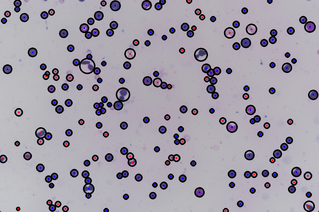
Finally, self clustering is carried out by Kmeans algorithm, which is divided into two categories and marked on the original graph
The classification effect is as follows

The marking effect is carried out on the image, in which the red dot is one type and the blue dot is one type

The complete code is as follows:

import cv2
import numpy as np
from skimage import measure,color
import collections
import matplotlib.pyplot as plt
from sklearn.cluster import KMeans

image_orign=cv2.imread(r'C:\Users\DELL\Desktop\1.jpg')
gray = cv2.cvtColor(image_orign,cv2.COLOR_BGR2GRAY)
blurred=cv2.GaussianBlur(gray,(11,11),0)
thresh=cv2.adaptiveThreshold(blurred, 255, cv2.ADAPTIVE_THRESH_MEAN_C, cv2.THRESH_BINARY_INV, 11, 2)
kernel=cv2.getStructuringElement(cv2.MORPH_ELLIPSE,(5,5))
erode_img=cv2.erode(thresh,kernel,iterations=1)#corrosion
dilate_img=cv2.dilate(erode_img,kernel,iterations=1)#expand

#watershed algorithm 
# sure_bg=cv2.dilate(dilate_img,kernel,iterations=3)#expand
# cv2.imshow('t',sure_bg)
# cv2.waitKey(0)
# dist_transform=cv2.distanceTransform(dilate_img,cv2.DIST_L2,5)
# ret ,sure_fg=cv2.threshold(dist_transform,0.55*dist_transform.max(),255,0)
# cv2.imshow('t',sure_fg)
# cv2.waitKey(0)
# sure_fg = np.uint8(sure_fg)
# unknow=cv2.subtract(sure_bg,sure_fg)
# ret2,makers=cv2.connectedComponents(sure_fg)
# markers=makers+1
# markers[unknow==0]=255
# markers=cv2.watershed(image_orign,markers)
# dilate_img[markers == 255] =0
# cv2.imshow('t',dilate_img)
# cv2.waitKey(0)

labels=measure.label(dilate_img,connectivity=2,background=1)
dst=color.label2rgb(labels)
image=np.zeros(dilate_img.shape,dtype='uint8')
cell_color=[]
for label in collections.Counter(np.unique(labels)).keys():
    if(label==1):
        continue
    mask=np.zeros(dilate_img.shape,dtype='uint8')
    mask[labels==label]=255
    num_pixel=cv2.countNonZero(mask)
    if(num_pixel>100):
        image=cv2.add(image,mask)

cell_set=[]
cell_size=[]
cont,hierarchy=cv2.findContours(image.copy(),cv2.RETR_EXTERNAL,cv2.CHAIN_APPROX_SIMPLE)
for i in cont:
    x,y,w,h=cv2.boundingRect(i)
    (cx,cy),radius=cv2.minEnclosingCircle(i)
    cv2.circle(image_orign,(int(cx),int(cy)),int(radius),(0,0,0),3)

    cell_set.append((int(cx),int(cy)))
    cell_size.append(np.pi*radius*radius/10)
    roi=np.zeros(gray.shape,dtype='uint8')
    roi = cv2.circle(roi, (int(cx),int(cy)), int(radius), 255, cv2.FILLED)
    mask2=np.ones(gray.shape,dtype='uint8')*255
    area=cv2.bitwise_and(mask2, gray, mask=roi)
    cell_color.append(area.sum()/cv2.countNonZero(area))

value=[]
d=cell_size.copy()
d.sort()
for i in d[len(d)-3:]:
    cell_set.pop(cell_size.index(i))
    cell_color.pop(cell_size.index(i))
    cell_size.remove(i)

for i in range(len(cell_set)):
    value.append([cell_size[i],cell_color[i]])
data=dict(zip(cell_set,value))
plt.scatter(cell_size,cell_color)
plt.show()

pre=KMeans(n_clusters=2).fit_predict(value)
c=[(255,0,0),(0,0,255)]
c2=['red','blue']
for i in range(len(list(pre))):
    plt.scatter(value[i][0],value[i][1],c=c2[pre[i]])
    cv2.circle(image_orign,(cell_set[i][0],cell_set[i][1]),3,c[pre[i]],cv2.FILLED)
cv2.imshow('t',image_orign)
cv2.waitKey(0)
plt.show()