Introduce

Numpy is an open source numerical calculation extension package for Python.

• Numpy supports common array and matrix operations. For the same numerical calculation task, using numpy is much simpler and more efficient than using Python directly.
• Numpy uses the ndarray object to handle multidimensional arrays, which is a fast and flexible big data container.
• Official website: https://numpy.org/

Numpy basic data structure ndarray

ndarray consists of two parts:

1. Actual data

2. Metadata describing these data

# Multidimensional array ndarray

import numpy as np

ar = np.array([1,2,3,4,5,6,7])
print(ar)          # Output the array. Pay attention to the format of the array: brackets. There is no comma between the elements (distinguished from the list)
print(ar.ndim)     # Output the number of array dimensions (number of axes), or "rank". The number of dimensions is also called rank
print(ar.shape)    # The dimension of the array. For an array with n rows and m columns, the shape is (n, m)
print(ar.size)     # The total number of elements of the array. For an array with n rows and m columns, the total number of elements is n*m
print(ar.dtype)    # The types of elements in the array are similar to type() (note that type() is a function and. dtype is a method)
print(ar.itemsize) # The byte size of each element in the array. The byte of int32l type is 4 and the byte of float64 is 8
print(ar.data)     # The buffer containing the actual array elements usually does not need to use this attribute because the elements are generally obtained through the index of the array.
ar   # Output in interactive mode, there will be array

# Basic properties of array
# ① The dimension of an array is called rank. The rank of a one-dimensional array is 1, the rank of a two-dimensional array is 2, and so on
# ② In NumPy, each linear array is called an axis, and the rank actually describes the number of axes:
# For example, a two-dimensional array is equivalent to two one-dimensional arrays, in which each element in the first one-dimensional array is a one-dimensional array
# Therefore, a one-dimensional array is the axes in NumPy. The first axis is equivalent to the underlying array, and the second axis is the array in the underlying array.
# The number of axes, the rank, is the dimension of the array. 

[1 2 3 4 5 6 7]
1
(7,)
7
int32
4
<memory at 0x0000021876391F40>





array([1, 2, 3, 4, 5, 6, 7])

Create an array (ndarray object)

1. Create ndarray objects using lists, primitives, arrays, and generators

2. np.arange() method creation

3. np.linspace() method creation

4. Through np internal specific methods

• zeros()
• zeros_like()
• ones()
• ones_like()
• eye()

# Create an array: array() function. The parentheses can be lists, primitives, arrays, generators, etc

ar1 = np.array(range(10))   # integer
ar2 = np.array([1,2,3.14,4,5])   # float 
# It can be any type, but it is not recommended to put non numeric data into numpy

ar3 = np.array([[1,2,3],('a','b','c')])   # Two dimensional array: nested sequence (list, Yuanzu)
ar4 = np.array([[1,2,3],('a','b','c','d')])   # Notice how the number of nested sequences varies 
print_info = lambda ar : print(ar,'\n',type(ar),'\n',ar.dtype,'\n',ar.ndim,'\n',ar.size,'\n','*'*30)

print_info(ar1)
print_info(ar2)
print_info(ar3)     # Two dimensional array, 6 elements in total, of Unicode type
print_info(ar4)     # A one-dimensional array with 2 elements in total. The elements are of object type

[0 1 2 3 4 5 6 7 8 9] 
 <class 'numpy.ndarray'> 
 int32 
 1 
 10 
 ******************************
[1.   2.   3.14 4.   5.  ] 
 <class 'numpy.ndarray'> 
 float64 
 1 
 5 
 ******************************
[['1' '2' '3']
 ['a' 'b' 'c']] 
 <class 'numpy.ndarray'> 
 <U11 
 2 
 6 
 ******************************
[list([1, 2, 3]) ('a', 'b', 'c', 'd')] 
 <class 'numpy.ndarray'> 
 object 
 1 
 2 
 ******************************


<ipython-input-23-2a69c3dbf06c>:8: VisibleDeprecationWarning: Creating an ndarray from ragged nested sequences (which is a list-or-tuple of lists-or-tuples-or ndarrays with different lengths or shapes) is deprecated. If you meant to do this, you must specify 'dtype=object' when creating the ndarray.
  ar4 = np.array([[1,2,3],('a','b','c','d')])   # Notice how the number of nested sequences varies

# Create an array: range(), similar to range(), and return evenly spaced values within a given interval.

print(np.arange(10))    # Returns 0-9, integer
print(np.arange(10.0))  # Return 0.0-9.0, floating point
print(np.arange(5,12))  # Return to 5-11
print(np.arange(5.0,12,2))  # Returns 5.0-12.0 in steps of 2
print(np.arange(10000))  # If the array is too large to print, NumPy will automatically skip the center of the array and print only the corners:

[0 1 2 3 4 5 6 7 8 9]
[ 0.  1.  2.  3.  4.  5.  6.  7.  8.  9.]
[ 5  6  7  8  9 10 11]
[  5.   7.   9.  11.]
[   0    1    2 ..., 9997 9998 9999]

# Create array: linspace(): returns num evenly spaced samples calculated on the interval [start, stop].

ar1 = np.linspace(2.0, 3.0, num=5)
ar2 = np.linspace(2.0, 3.0, num=5, endpoint=False)
ar3 = np.linspace(2.0, 3.0, num=5, retstep=True)
print(ar1,type(ar1))
print(ar2)
print(ar3,type(ar3))
# numpy.linspace(start, stop, num=50, endpoint=True, retstep=False, dtype=None)
# Start: start value, stop: end value
# num: number of generated samples; the default value is 50
# endpoint: if True, the stop is the last sample. Otherwise, it is not included. The default value is True.
# retstep: if true, return (sample, step), where step is the spacing between samples → output is a primitive containing two elements, the first element is array, and the second is the actual value of step

[ 2.    2.25  2.5   2.75  3.  ] <class 'numpy.ndarray'>
[ 2.   2.2  2.4  2.6  2.8]
(array([ 2.  ,  2.25,  2.5 ,  2.75,  3.  ]), 0.25) <class 'tuple'>

# Create array: zeros()/zeros_like()/ones()/ones_like()

ar1 = np.zeros(5)  
ar2 = np.zeros((2,2), dtype = np.int)
print(ar1,ar1.dtype)
print(ar2,ar2.dtype)
print('------')
# numpy.zeros(shape, dtype=float, order='C '): returns a new array of the given shape and type, filled with zeros.
# shape: array dimension. If it is more than two dimensions, use (), and the input parameter is an integer
# dtype: data type, default numpy float64
# order: whether to store multidimensional data in memory in C or Fortran continuously (in rows or columns).

ar3 = np.array([list(range(5)),list(range(5,10))])
ar4 = np.zeros_like(ar3)
print(ar3)
print(ar4)
print('------')
# Returns a zero array with the same shape and type as the given array, where ar4 creates an array of all zeros according to the shape and dtype of ar3

ar5 = np.ones(9)
ar6 = np.ones((2,3,4))
ar7 = np.ones_like(ar3)
print(ar5)
print(ar6)
print(ar7)
# ones()/ones_like() and zeros()/zeros_like(), but filled with 1

[ 0.  0.  0.  0.  0.] float64
[[0 0]
 [0 0]] int32
------
[[0 1 2 3 4]
 [5 6 7 8 9]]
[[0 0 0 0 0]
 [0 0 0 0 0]]
------
[ 1.  1.  1.  1.  1.  1.  1.  1.  1.]
[[[ 1.  1.  1.  1.]
  [ 1.  1.  1.  1.]
  [ 1.  1.  1.  1.]]

 [[ 1.  1.  1.  1.]
  [ 1.  1.  1.  1.]
  [ 1.  1.  1.  1.]]]
[[1 1 1 1 1]
 [1 1 1 1 1]]

# Create array: eye()

print(np.eye(5))
# Create a square N*N identity matrix with diagonal value of 1 and the rest of 0

[[ 1.  0.  0.  0.  0.]
 [ 0.  1.  0.  0.  0.]
 [ 0.  0.  1.  0.  0.]
 [ 0.  0.  0.  1.  0.]
 [ 0.  0.  0.  0.  1.]]

Data type of ndarray

bool a boolean type (True or False) stored in one byte

inti is an integer whose size is determined by the platform (generally int32 or int64)

int8 one byte size, - 128 to 127

int16 integer, - 32768 to 32767

int32 integer, - 2 * * 31 to 2 * * 32 - 1

int64 integer, - 2 * * 63 to 2 * * 63 - 1

uint8 unsigned integer, 0 to 255

uint16 unsigned integer, 0 to 65535

uint32 unsigned integer, 0 to 2 * * 32 - 1

uint64 unsigned integer, 0 to 2 * * 64 - 1

float16 semi precision floating point number: 16 bits, 1 sign, 5 exponent and 10 precision

float32 single precision floating point number: 32 bits, sign 1 bit, exponent 8 bits, precision 23 bits

float64 or float double precision floating point number: 64 bits, sign 1 bit, exponent 11 bits, precision 52 bits

complex64 complex number, which uses two 32-bit floating-point numbers to represent the real part and imaginary part respectively

complex128 or complex complex complex numbers, which represent the real part and imaginary part with two 64 bit floating-point numbers respectively

Numpy general function

Basic operation 1

• np.T
• np.reshape() provides a new shape for the array. The total number should be consistent
• np.resize() returns a new array with the specified shape, which can be repeated if necessary
• np.copy()
• np.astype()

Basic operation 2

• np. Stack
• np.vstack() stacks arrays horizontally (in row order)
• np. Hsstack() stacks arrays vertically (in column order)
• np. Split
• np.vsplit() splits the array horizontally (in row order)
• np.hsplit() splits the array vertically (in row order)

# Array shape: T/.reshape()/.resize()

ar1 = np.arange(10)
ar2 = np.ones((5,2))
print(ar1,'\n',ar1.T,ar1.shape,ar1.T.shape)
print(ar2,'\n',ar2.T)
print('-'*50)
# . T method: transpose. For example, the original shape is (3,4) / (2,3,4), and the transpose result is (4,3) / (4,3,2) → therefore, the result of one-dimensional array transpose remains unchanged

ar3 = ar1.reshape(2,5)     # Usage 1: directly change the shape of the existing array             
ar4 = np.zeros((4,6)).reshape(3,8)   # Usage 2: directly change the shape after generating the array
# np.zeros((4,6)).reshape(4,8) #cannot reshape array of size 24 into shape (4,8)

ar5 = np.reshape(np.arange(12),(3,4))   # Usage 3: add an array and target shape to the parameter
print('\nar1\n',ar1,'\nar3\n',ar3)
print(ar4)
print(ar5)
print('-'*50)
# numpy.reshape(a, newshape, order='C '): provide a new shape for the array without changing its data, so the number of elements needs to be consistent!!

ar6 = np.resize(np.arange(5),(3,4))
print(ar6)
# numpy.resize(a, new_shape): returns a new array with the specified shape. If necessary, the required number of elements can be filled repeatedly.
# Note: T/.reshape()/.resize() generates new arrays!!!
print(ar1 is ar1.T)

[0 1 2 3 4 5 6 7 8 9] 
 [0 1 2 3 4 5 6 7 8 9] (10,) (10,)
[[1. 1.]
 [1. 1.]
 [1. 1.]
 [1. 1.]
 [1. 1.]] 
 [[1. 1. 1. 1. 1.]
 [1. 1. 1. 1. 1.]]
--------------------------------------------------

ar1
 [0 1 2 3 4 5 6 7 8 9] 
ar3
 [[0 1 2 3 4]
 [5 6 7 8 9]]
[[0. 0. 0. 0. 0. 0. 0. 0.]
 [0. 0. 0. 0. 0. 0. 0. 0.]
 [0. 0. 0. 0. 0. 0. 0. 0.]]
[[ 0  1  2  3]
 [ 4  5  6  7]
 [ 8  9 10 11]]
--------------------------------------------------
[[0 1 2 3]
 [4 0 1 2]
 [3 4 0 1]]
False

# Copy of array copy()

old_ar = np.arange(10)
new_ar = old_ar
print(new_ar is old_ar)
new_ar[2] = 9
print('\nnew_ar:\n',new_ar,'\nold_ar:\n',old_ar)
# Recall python's assignment logic: point to a value generated in memory → here ar1 and ar2 point to the same value, so ar1 changes and ar2 changes together

copy_new_ar = ar1.copy()
print(copy_new_ar is old_ar)
copy_new_ar[0] = 9
print('\ncopy_new_ar:\n',copy_new_ar,'\nold_ar:\n',old_ar,)
# The copy method generates a full copy of the array and its data
# Remind again: T/.reshape()/.resize() generates new arrays!!!

True

new_ar:
 [0 1 9 3 4 5 6 7 8 9] 
old_ar:
 [0 1 9 3 4 5 6 7 8 9]
False

copy_new_ar:
 [9 1 9 3 4 5 6 7 8 9] 
old_ar:
 [0 1 9 3 4 5 6 7 8 9]

# Array type conversion: astype()

ar1 = np.arange(10,dtype=float)
print(ar1,ar1.dtype)
print('-----')
# You can set the array type at the parameter position

ar2 = ar1.astype(np.int32)
print(ar2,ar2.dtype)
print(ar1,ar1.dtype)
# a.astype(): convert array type
# Note: get into the habit of using NP. For array types Int32 instead of int32 directly

[ 0.  1.  2.  3.  4.  5.  6.  7.  8.  9.] float64
-----
[0 1 2 3 4 5 6 7 8 9] int32
[ 0.  1.  2.  3.  4.  5.  6.  7.  8.  9.] float64

# Array stack

# numpy.hstack(tup): stacks arrays horizontally (in column order)
a = np.arange(5)    # A is a one-dimensional array with 5 elements
b = np.arange(5,9) # b is a one-dimensional array with 4 elements
ar1 = np.hstack((a,b))  # Note: ((a,b)), the shape here can be different
print(a,a.shape)
print(b,b.shape)
print(ar1,ar1.shape)
a = np.array([[1],[2],[3]])   # A is a two-dimensional array with 3 rows and 1 column
b = np.array([['a'],['b'],['c']])  # b is a two-dimensional array, 3 rows and 1 column
ar2 = np.hstack((a,b))  # Note: ((a,b)), the shape here must be the same
print(a,a.shape)
print(b,b.shape)
print(ar2,ar2.shape)

[0 1 2 3 4] (5,)
[5 6 7 8] (4,)
[0 1 2 3 4 5 6 7 8] (9,)
[[1]
 [2]
 [3]] (3, 1)
[['a']
 ['b']
 ['c']] (3, 1)
[['1' 'a']
 ['2' 'b']
 ['3' 'c']] (3, 2)

# numpy.vstack(tup): stacks arrays vertically (in column order)
a = np.arange(5)    
b = np.arange(5,10)
ar1 = np.vstack((a,b))
print(a,a.shape)
print(b,b.shape)
print(ar1,ar1.shape)
a = np.array([[1],[2],[3]])   
b = np.array([['a'],['b'],['c'],['d']])   
ar2 = np.vstack((a,b))  # The shape here can be different
print(a,a.shape)
print(b,b.shape)
print(ar2,ar2.shape)

[0 1 2 3 4] (5,)
[5 6 7 8 9] (5,)
[[0 1 2 3 4]
 [5 6 7 8 9]] (2, 5)
[[1]
 [2]
 [3]] (3, 1)
[['a']
 ['b']
 ['c']
 ['d']] (4, 1)
[['1']
 ['2']
 ['3']
 ['a']
 ['b']
 ['c']
 ['d']] (7, 1)

# numpy.stack(arrays, axis=0): connect the array sequence along the new axis. The shape must be the same!
# Focus on explaining the meaning of the axis parameter. Suppose two arrays [1,2,3] and [4,5,6], and the shape is (3,0)

a = np.arange(5)    
b = np.arange(5,10)
ar1 = np.stack((a,b))
ar2 = np.stack((a,b),axis = 1)
print(a,a.shape)
print(b,b.shape)
print(ar1,ar1.shape)
print(ar2,ar2.shape)
# axis=0: [[1 2 3] [4 5 6]], shape is (2,3)
# axis=1: [[1 4] [2 5] [3 6]], shape is (3,2)

[0 1 2 3 4] (5,)
[5 6 7 8 9] (5,)
[[0 1 2 3 4]
 [5 6 7 8 9]] (2, 5)
[[0 5]
 [1 6]
 [2 7]
 [3 8]
 [4 9]] (5, 2)

# Array splitting 
# Note: the input is nparray, the output result is list, and the elements in the list are arrays
# numpy. Hsplit (ary, indexes_or_sections): split the array horizontally (column by column) into multiple sub arrays → split by column
ar = np.arange(16).reshape(4,4)
ar1 = np.split(ar,indices_or_sections=2,axis=1)
ar2 = np.hsplit(ar,2)
print(ar)
print(ar1,'\n',type(ar1))
print(ar2,'\n',type(ar2))

[[ 0  1  2  3]
 [ 4  5  6  7]
 [ 8  9 10 11]
 [12 13 14 15]]
[array([[ 0,  1],
       [ 4,  5],
       [ 8,  9],
       [12, 13]]), array([[ 2,  3],
       [ 6,  7],
       [10, 11],
       [14, 15]])] 
 <class 'list'>
[array([[ 0,  1],
       [ 4,  5],
       [ 8,  9],
       [12, 13]]), array([[ 2,  3],
       [ 6,  7],
       [10, 11],
       [14, 15]])] 
 <class 'list'>

# numpy.vsplit(ary, indices_or_sections): split the array vertically (row direction) into multiple sub arrays → split by row
ar2 = np.vsplit(ar,4)
print(ar)
print(ar2,type(ar2))

[[ 0  1  2  3]
 [ 4  5  6  7]
 [ 8  9 10 11]
 [12 13 14 15]]
[array([[0, 1, 2, 3]]), array([[4, 5, 6, 7]]), array([[ 8,  9, 10, 11]]), array([[12, 13, 14, 15]])] <class 'list'>

Simple operation of numpy array

Addition, subtraction, multiplication, division, remainder, modulus and power

• np.mean() average

• np. Max (max)

• np. Min (min)

• np.std() standard deviation

• np. Var (variance)

• np.sum()

• np.sort() sort

# Array simple operation

ar = np.arange(6).reshape(2,3)
print(ar + 10)   # addition
print(ar * 2)   # multiplication
print(1 / (ar+1))  # division
print(ar ** 0.5)  # power
# Operation with scalar

print(ar.mean())  # Average
print(ar.max())  # Find the maximum value
print(ar.min())  # Find the minimum value
print(ar.std())  # Standard deviation
print(ar.var())  # Find variance
print(ar.sum(), np.sum(ar,axis = 0))  # Sum, NP Sum() → axis is 0, sum by column; Axis is 1, sum by line
print(np.sort(np.array([1,4,3,2,5,6])))  # sort
# Common functions

[[10 11 12]
 [13 14 15]]
[[ 0  2  4]
 [ 6  8 10]]
[[1.         0.5        0.33333333]
 [0.25       0.2        0.16666667]]
[[0.         1.         1.41421356]
 [1.73205081 2.         2.23606798]]
2.5
5
0
1.707825127659933
2.9166666666666665
15 [3 5 7]
[1 2 3 4 5 6]

########There are assignments for this class. Please check "course assignments. docx"########

Numpy index and slice

• Basic index and slice
• Boolean index and slice

'''
[Course 1.4]  Numpy Index and slice

Core: basic index and slice / Boolean index and slice

'''

# Basic index and slice

# One dimensional array index and slice
ar = np.arange(20)
print(ar)
print(ar[4])
print(ar[3:6])
print('-----')

[ 0  1  2  3  4  5  6  7  8  9 10 11 12 13 14 15 16 17 18 19]
4
[3 4 5]
-----

# Two dimensional array index and slice
ar = np.arange(16).reshape(4,4)
print(ar, 'The number of array axes is%i' %ar.ndim,'\n')   # 4 * 4 array
print(ar[2],  'The number of array axes is%i' %ar[2].ndim,'\n')  # The slice is an element of the next dimension, so it is a one-dimensional array
print(ar[2][1]) # Secondary index to get a value in a one-dimensional array
print(ar[1:3],  'The number of array axes is%i' %ar[1:3].ndim,'\n')  # The slice is a two-dimensional array composed of two one-dimensional arrays
print(ar[2,2])  # The third row and the third column in the slice array → 10
print(ar[:2,1:])  # 1,2 rows, 2,3,4 columns in slice array → 2D array

[[ 0  1  2  3]
 [ 4  5  6  7]
 [ 8  9 10 11]
 [12 13 14 15]] The number of array axes is 2 

[ 8  9 10 11] The number of array axes is 1 

9
[[ 4  5  6  7]
 [ 8  9 10 11]] The number of array axes is 2 

10
[[1 2 3]
 [5 6 7]]

# **3D array index and slice
ar = np.arange(8).reshape(2,2,2)
print(ar, 'The number of array axes is%i' %ar.ndim,'\n')   # 2 * 2 * 2 array
print(ar[0],  'The number of array axes is%i' %ar[0].ndim,'\n')  # The first element of the next dimension of a 3D array → a 2D array
print(ar[0][0],  'The number of array axes is%i' %ar[0][0].ndim,'\n')  # First element under the first element of the next dimension of a three-dimensional array → a one-dimensional array
print(ar[0][0][1],  'The number of array axes is%i' %ar[0][0][1].ndim,'\n')  

[[[0 1]
  [2 3]]

 [[4 5]
  [6 7]]] The number of array axes is 3 

[[0 1]
 [2 3]] The number of array axes is 2 

[0 1] The number of array axes is 1 

1 The number of array axes is 0 

# Boolean index and slice

ar = np.arange(12).reshape(3,4)
i = np.array([True,False,True])
j = np.array([True,True,False,False])
print(ar)
print(i)
print(j)
print(ar[i,:])  # Judge in the first dimension and only keep True. Here, the first dimension is the row, ar[i,:] = ar[i] (simple writing format)
print(ar[:,j])  # In the second dimension, if ar[:,i] is judged, there will be a warning, because i is three elements and AR has four elements in the column
# Boolean index: filter by Boolean matrix

m = ar > 5
print(m)  # Here m is a judgment matrix
print(ar[m])  # Filter elements > 5 in ar array with m judgment matrix → key! The later principle of pandas judgment comes from here

[[ 0  1  2  3]
 [ 4  5  6  7]
 [ 8  9 10 11]]
[ True False  True]
[ True  True False False]
[[ 0  1  2  3]
 [ 8  9 10 11]]
[[0 1]
 [4 5]
 [8 9]]
[[False False False False]
 [False False  True  True]
 [ True  True  True  True]]
[ 6  7  8  9 10 11]

# Change and copy the value of array index and slice

ar = np.arange(10)
print(ar)
ar[5] = 100
ar[7:9] = 200
print(ar)
# When a scalar is assigned to an index / slice, the original array is automatically changed / propagated

ar = np.arange(10)
b = ar.copy()
b[7:9] = 200
print(ar)
print(b)
# copy

[0 1 2 3 4 5 6 7 8 9]
[  0   1   2   3   4 100   6 200 200   9]
[0 1 2 3 4 5 6 7 8 9]
[  0   1   2   3   4   5   6 200 200   9]

########There are assignments for this class. Please check "course assignments. docx"########

Numpy random number

• np.random.normal standard normal distribution
• np.random.rand random distribution

'''
[Course 1.5]  Numpy random number

numpy.random Random samples with multiple probability distributions are one of the key tools for data analysis

'''

'[Course 1.5]  Numpy random number\n\nnumpy.random Random samples with multiple probability distributions are one of the key tools for data analysis'

# generation of random number

samples = np.random.normal(size=(4,4))
print(samples)
# Generate a 4 * 4 sample value of standard positive Pacific distribution

[[ 0.62264655  0.61998157  0.32688731  1.77734136]
 [-0.57888784 -2.32079299  0.52235571 -0.86664107]
 [-0.50608591  0.97127901  1.29301905  0.70268877]
 [-1.17447292  0.24604616 -2.36537572 -1.66786748]]

# numpy. random. Rand (d0, D1,..., DN): generate a random floating-point number or N-dimensional floating-point array between [0,1) -- uniform distribution

import matplotlib.pyplot as plt  # Import the matplotlib module for chart auxiliary analysis


a = np.random.rand()
print(a,type(a))  # Generate a random floating point number

b = np.random.rand(4)
print(b,type(b))  # Generate a one-dimensional array of shape 4

c = np.random.rand(2,3)
print(c,type(c))  # Generate a two-dimensional array with a shape of 2 * 3. Note that this is not ((2,3))

0.6013530120068452 <class 'float'>
[0.73744877 0.9389245  0.17095026 0.34667055] <class 'numpy.ndarray'>
[[0.32994562 0.41394496 0.03012815]
 [0.8541199  0.99239343 0.96816951]] <class 'numpy.ndarray'>

samples1 = np.random.rand(1000)
samples2 = np.random.rand(1000)
plt.scatter(samples1,samples2)
# Generate 1000 uniformly distributed sample values

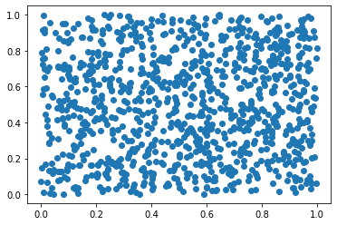
<matplotlib.collections.PathCollection at 0x2187646f3d0>

#  Numpy.random.randn (d0, D1,..., DN): generate a floating-point number or N-dimensional floating-point array - normal distribution

samples1 = np.random.randn(1000)
samples2 = np.random.randn(1000)
plt.scatter(samples1,samples2)
# The parameters randn and rand are used in the same way
# Generate 1000 normal sample values

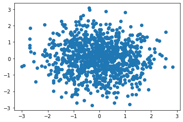
<matplotlib.collections.PathCollection at 0x21876314850>

# Numpy. Random. Random (low, high = none, size = none, dtype ='l '): generates an integer or N-dimensional integer array
# If high is not None, take the random integer between [low, high], otherwise take the random integer between [0,low), and high must be greater than low 
# dtype parameter: can only be of type int  

# low=2: generate 1 random integer between [0,2] 
print(np.random.randint(2))
 

# low=2,size=5: generate 5 random integers between [0,2]
print(np.random.randint(2,size=5))

# low=2,high=6,size=5: generate 5 random integers between [2,6]  
print(np.random.randint(2,6,size=5))

# low=2,size=(2,3): generate an array of 2x3 integers, and the fetching range is: [0,2) random integers 
print(np.random.randint(2,size=(2,3)))

# low=2,high=6,size=(2,3): generate a 2 * 3 integer array, value range: [2,6) random integer  
print(np.random.randint(2,6,(2,3)))

1
[1 0 0 1 1]
[2 5 5 5 4]
[[1 1 1]
 [1 1 0]]
[[2 5 3]
 [4 5 5]]

########There are assignments for this class. Please check "course assignments. docx"########

numpy data saving and loading

• np.save(file, arr)
• np.load(file,encoding='ASCII')
• np.savetxt()
• np.loadtxt()

'''
[Course 1.6]  Numpy Input and output of data

numpy read/Write array data and text data

'''

# Store array data. npy file

import os
os.chdir(r'E:\TempData') # Make current path

ar = np.random.rand(5,5)
print(ar)
np.save('arraydata.npy', ar)
# You can also directly np.save('C:/Users/Hjx/Desktop/arraydata.npy', ar)

[[0.32901445 0.82676533 0.51601218 0.28436385 0.45602576]
 [0.8253198  0.75243769 0.36862559 0.91892802 0.69506116]
 [0.88082892 0.55051927 0.73288251 0.61477109 0.91668244]
 [0.10730108 0.86434393 0.52938733 0.30694539 0.47642341]
 [0.33655539 0.41776535 0.44761788 0.01315365 0.1324372 ]]

# Read array data. npy file

ar_load =np.load('arraydata.npy')
print(ar_load)
# You can also directly np.load('C:/Users/Hjx/Desktop/arraydata.npy ')

[[0.32901445 0.82676533 0.51601218 0.28436385 0.45602576]
 [0.8253198  0.75243769 0.36862559 0.91892802 0.69506116]
 [0.88082892 0.55051927 0.73288251 0.61477109 0.91668244]
 [0.10730108 0.86434393 0.52938733 0.30694539 0.47642341]
 [0.33655539 0.41776535 0.44761788 0.01315365 0.1324372 ]]

# Store / read text files

ar = np.random.rand(5,5)
np.savetxt('array.txt',ar, delimiter=',')
# np.savetxt(fname, X, fmt='%.18e', delimiter=' ', newline='\n', header='', footer='', comments='# '): stored as a text txt file

ar_loadtxt = np.loadtxt('array.txt', delimiter=',')
print(ar_loadtxt)
# You can also directly NP. Loadtext ('c: / users / HJX / desktop / array. TXT ')

[[ 0.28280684  0.66188985  0.00372083  0.54051044  0.68553963]
 [ 0.9138449   0.37056825  0.62813711  0.83032184  0.70196173]
 [ 0.63438739  0.86552157  0.68294764  0.2959724   0.62337767]
 [ 0.67411154  0.87678919  0.53732168  0.90366896  0.70480366]
 [ 0.00936579  0.32914898  0.30001813  0.66198967  0.04336824]]

########There are assignments for this class. Please check "course assignments. docx"########