Correlation analysis is a way to find interesting connections in transaction data, such as the famous "beer diaper". Frequent sequence pattern mining can predict purchase behavior, biological sequence and so on.
10.2 converting data into transactions
Convert linked lists, matrices, and data frames into transactions
# Convert data into transactions
install.packages("arules")
library(arules)
tr_list <- list(c("Apple", "Bread", "Cake"),
                c("Apple", "Bread", "Milk"),
                c("Apple", "Cake", "Milk"))
names(tr_list) <- paste("Tr",c(1:3), sep = "")
trans <- as(tr_list, "transactions");trans
tr_matrix <- matrix(
  c(1,1,1,0,
    1,1,0,1,
    0,1,1,1),ncol = 4
)
dimnames(tr_matrix) <- list(
  paste("Tr",c(1:3), sep = ""),
  c("Apple", "Bread", "Cake", "Milk")
)
trans2 <- as(tr_matrix, "transactions");trans2
Tr_df <- data.frame(
  TrID = as.factor(c(1,2,1,1,2,3,2,3,2,3)),
  Item = as.factor(c("Apple", "Milk", "Cake", "Bread",
                     "Cake", "Milk", "Apple", "Cake",
                     "Bread", "Bread"))
)
trans3 <- as(split(Tr_df[,"Item"], Tr_df[,"TrID"]),
             "transactions");trans3
Calling the as function to add an id to each transaction completes the type conversion from data to transaction. "transactions" type represents transactional data of rules or frequent itemsets, which is an extension of itemMatrix type.
10.3 display affairs and related matters
The package type arr is used to store the data of its own transaction type.
LIST(trans) # Display data in list form
$Tr1
[1] "Apple" "Bread" "Cake"
$Tr2
[1] "Apple" "Bread" "Milk"
$Tr3
[1] "Apple" "Cake" "Milk"
summary(trans)
transactions as itemMatrix in sparse format with
3 rows (elements/itemsets/transactions) and
4 columns (items) and a density of 0.75
most frequent items:
Apple Bread Cake Milk (Other)
3 2 2 2 0
element (itemset/transaction) length distribution:
sizes
3
3
Min. 1st Qu. Median Mean 3rd Qu. Max.
3 3 3 3 3 3
includes extended item information - examples:
labels
1 Apple
2 Bread
3 Cake
includes extended transaction information - examples:
transactionID
1 Tr1
2 Tr2
3 Tr3
inspect(trans)
items transactionID
[1] {Apple, Bread, Cake} Tr1
[2] {Apple, Bread, Milk} Tr2
[3] {Apple, Cake, Milk} Tr3
filter_trans <- trans[size(trans) >=3]
inspect(filter_trans)
items transactionID
[1] {Apple, Bread, Cake} Tr1
[2] {Apple, Bread, Milk} Tr2
[3] {Apple, Cake, Milk} Tr3
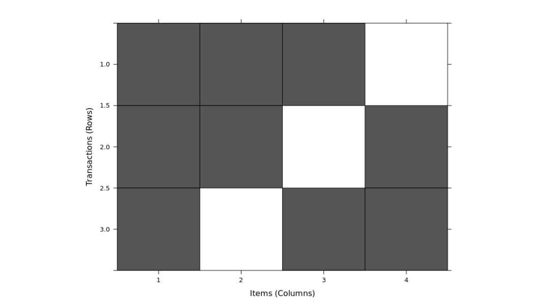
image(trans)
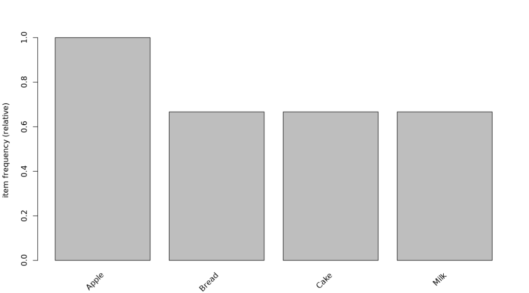
itemFrequencyPlot(trans)
itemFrequency(trans) # Distribution of support
Apple Bread Cake Milk
1.0000000 0.6666667 0.6666667 0.6666667
10.4 association mining based on Apriori rules
First find the frequent individual itemsets, and then generate larger frequent itemsets through breadth first search strategy.
data("Groceries")
summary(Groceries)
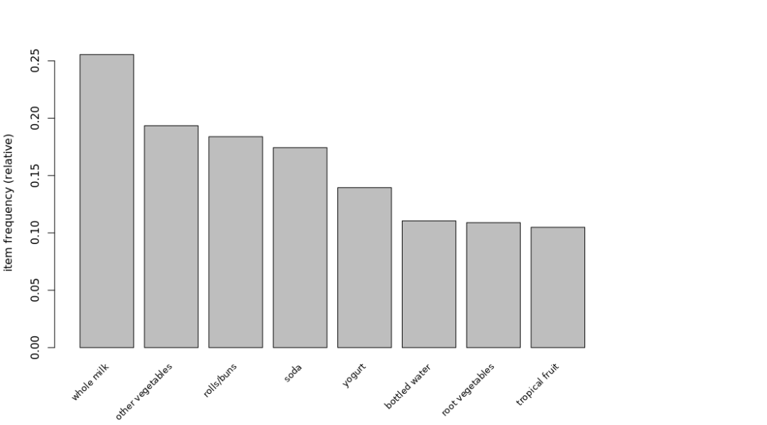
itemFrequencyPlot(Groceries,support=0.1, cex.names=0.8, topN=10)
rules <- apriori(Groceries, parameter = list(supp=0.001, conf=0.5,
target="rules"))
summary(rules)
inspect(head(rules))
lhs rhs support confidence coverage lift count
[1] {honey} => {whole milk} 0.001118454 0.7333333 0.001525165 2.870009 11
[2] {tidbits} => {rolls/buns} 0.001220132 0.5217391 0.002338587 2.836542 12
[3] {cocoa drinks} => {whole milk} 0.001321810 0.5909091 0.002236909 2.312611 13
[4] {pudding powder} => {whole milk} 0.001321810 0.5652174 0.002338587 2.212062 13
[5] {cooking chocolate} => {whole milk} 0.001321810 0.5200000 0.002541942 2.035097 13
[6] {cereals} => {whole milk} 0.003660397 0.6428571 0.005693950 2.515917 36
rules <- sort(rules, by="confidence", decreasing = TRUE)
inspect(head(rules))
lhs rhs support confidence coverage lift count
[1] {rice,
sugar} => {whole milk} 0.001220132 1 0.001220132 3.913649 12
[2] {canned fish,
hygiene articles} => {whole milk} 0.001118454 1 0.001118454 3.913649 11
[3] {root vegetables,
butter,
rice} => {whole milk} 0.001016777 1 0.001016777 3.913649 10
[4] {root vegetables,
whipped/sour cream,
flour} => {whole milk} 0.001728521 1 0.001728521 3.913649 17
[5] {butter,
soft cheese,
domestic eggs} => {whole milk} 0.001016777 1 0.001016777 3.913649 10
[6] {citrus fruit,
root vegetables,
soft cheese} => {other vegetables} 0.001016777 1 0.001016777 5.168156 10
>
The strength of rules can be evaluated by two values: support and association. The former represents the frequency of rules and represents the probability that two itemsets appear in a transaction at the same time. These two indicators are only effective for judging the strength of rules, and some rules may also be redundant. The promotion degree can evaluate the quality of rules. The degree of support represents the proportion in the transaction database of a specific item set. The degree of confidence is the accuracy of the rule, and the degree of promotion is the ratio of the response target association rule to the average response. Apriori is the most well-known association rule mining algorithm, which relies on the breadth first strategy layer by layer to generate the candidate set. You can also call the intersectMeasure function to get other interesting metrics.
head(interestMeasure(rules,c("support", "chiSquare", "confidence",
+                              "conviction", "cosine", "coverage",
+                              "leverage", "lift", "oddsRatio"),
+                      Groceries))
      support chiSquared confidence conviction     cosine    coverage     leverage     lift
1 0.001220132   35.00650          1        Inf 0.06910260 0.001220132 0.0009083689 3.913649
2 0.001118454   32.08603          1        Inf 0.06616070 0.001118454 0.0008326715 3.913649
3 0.001016777   29.16615          1        Inf 0.06308175 0.001016777 0.0007569741 3.913649
4 0.001728521   49.61780          1        Inf 0.08224854 0.001728521 0.0012868559 3.913649
5 0.001016777   29.16615          1        Inf 0.06308175 0.001016777 0.0007569741 3.913649
6 0.001016777   41.72398          1        Inf 0.07249042 0.001016777 0.0008200380 5.168156
  oddsRatio
1       Inf
2       Inf
3       Inf
4       Inf
5       Inf
6       Inf
10.5 remove redundancy rules
The two main limitations of association rule mining are the choice between support and confidence, de redundancy and finding the really meaningful information in these rules. I don't know much about this field at the beginning. I'll put it here first.
# derep
rules.sorted <- sort(rules, by="lift")
subset.matrix <- is.subset(rules.sorted, rules.sorted)
subset.matrix[lower.tri(subset.matrix, diag=T)] <- NA
redundant <- colSums(subset.matrix, na.rm=TRUE) >= 8
rules.pruned <- rules.sorted[!redundant]
inspect(head(rules.pruned))
    lhs                   rhs              support confidence    coverage     lift count
[1] {citrus fruit,
     pip fruit,
     bottled water}    => {whole milk} 0.001118454        0.5 0.002236909 1.956825    11
[2] {citrus fruit,
     pip fruit,
     yogurt}           => {whole milk} 0.001626843        0.5 0.003253686 1.956825    16
[3] {root vegetables,
     rolls/buns,
     soda}             => {whole milk} 0.002440264        0.5 0.004880529 1.956825    24
[4] {tropical fruit,
     other vegetables,
     rolls/buns,
     soda}             => {whole milk} 0.001118454        0.5 0.002236909 1.956825    11
It is found that there are no rules that survive according to the original book > = 1. After reading it, if it is set to more than 4, there will be 8. It is found that computers with small memory may crash in this step, because the matrix is large. For example, small cloud hosts can run successfully on computers with 16G memory.
10.6 visualization of association rules
Reset it to 1800 for visual beauty
install.packages("arulesViz")
library(arulesViz)
install.packages('Rcpp')
library(Rcpp) #If this package is found to be installed, it will be reported as Error in stress_major(xinit, W, D, iter, tol) :
function 'Rcpp_precious_remove' not provided by package 'Rcpp'
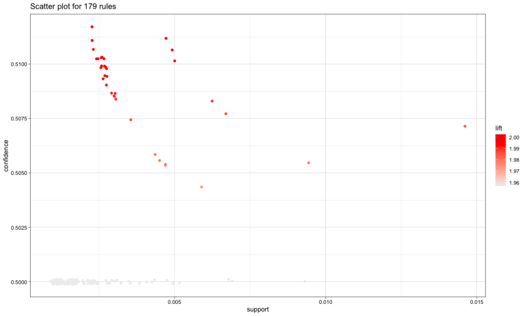
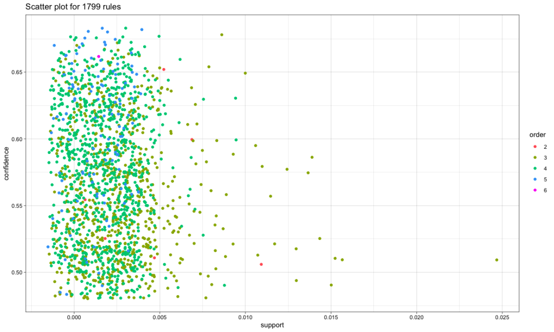
plot(rules.pruned)
#Avoid overlap and shake
plot(rules.pruned,shading='order', control =list(jitter=6))
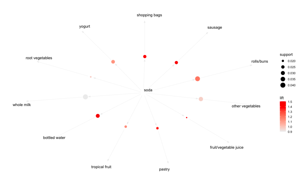
# Apriori algorithm generates new rules with soda on the left
soda_rule <- apriori(data = Groceries, parameter = list(supp=0.001,conf=0.1,minlen=2),
appearance = list(default='rhs',lhs='soda'))
plot(sort(soda_rule,by="lift"), method = 'graph',
control = list(type='items'))
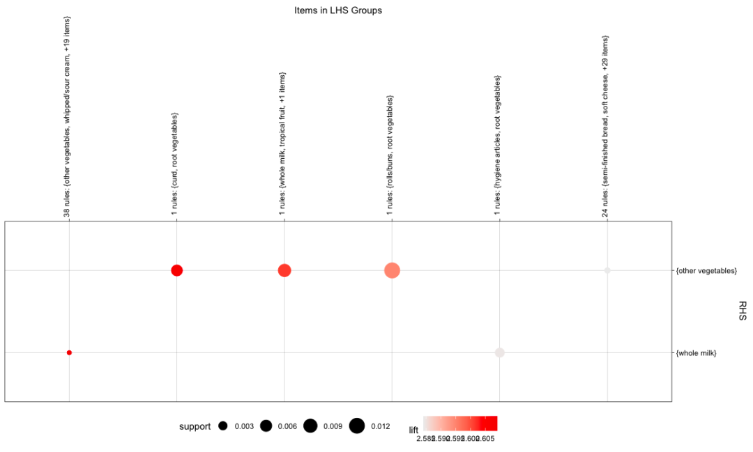
plot(rules.pruned[c(1:66)],method="group") # It is reported here:
Error in stats::hclust(stats::dist(m_clust)) :
must have n >= 2 objects to cluster
So use the one in the previous step instead
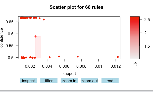
Interactive graphic plot(rules.pruned[c(1:66)],interactive = TRUE)
10.7 mining frequent itemsets using Eclat
Apriori algorithm uses breadth first strategy to traverse the database, which takes a long time; If the database can be loaded into memory, the depth first Eclat algorithm can be used, which is more efficient than the former.
# Eclat
frequentest <- eclat(Groceries, parameter = list(support=0.05,maxlen=10))
summary(frequentest)
inspect(sort(frequentest, by="support")[1:10])
     items              support    count
[1]  {whole milk}       0.25551601 2513
[2]  {other vegetables} 0.19349263 1903
[3]  {rolls/buns}       0.18393493 1809
[4]  {soda}             0.17437722 1715
[5]  {yogurt}           0.13950178 1372
[6]  {bottled water}    0.11052364 1087
[7]  {root vegetables}  0.10899847 1072
[8]  {tropical fruit}   0.10493137 1032
[9]  {shopping bags}    0.09852567  969
[10] {sausage}          0.09395018  924
Apriori algorithm is direct and easy to understand. The disadvantage is that it needs to scan the database many times, so it will produce a large number of candidate sets, and the calculation of support is very time-consuming. Eclat algorithm adopts the strategies of equivalence class, depth first traversal and subordination, which greatly improves the efficiency of support calculation. The former uses the horizontal data structure to store transactions, while the latter uses the vertical data structure to store the transaction ID of each transaction, and also generates association rules from the frequent item set. FP growth is also a widely used association rule mining algorithm, which is similar to Eclat algorithm. It also uses the deep first search strategy to calculate the itemset support. There is no package support for the time being? 2021, maybe.
10.8 generating temporal transaction data
# tense
install.packages("arulesSequences")
library(arulesSequences)
tmp_data <- list(
  c("A"),
  c("A","B","C"),
  c("D"),
  c("c","F"),
  c("A","D"),
  c("C"),
  c("B", "C"),
  c("A","E"),
  c("E","F"),
  c("A","B"),
  c("D","F"),
  c("C"),
  c("B"),
  c("E"),
  c("G"),
  c("A","F"),
  c("C"),
  c("B"),
  c("C")
)
# Convert to transaction
names(tmp_data) <- paste0("Tr", c(1:19), seq="")
trans <- as(tmp_data, "transactions")
transactionInfo(trans)$SequenceID <- c(1,1,1,1,1,2,2,2,2,3,3,3,3,3,4,4,4,4,4)
transactionInfo(trans)$eventID<- c(10,20,30,40,50,10,20,30,40,10,20,30,40,50,
                                   10,20,30,40,50)
trans
transactions in sparse format with
 19 transactions (rows) and
 8 items (columns)
inspect(head(trans))
    items   transactionID eventID
[1] {A}     Tr1           10
[2] {A,B,C} Tr2           20
[3] {D}     Tr3           30
[4] {c,F}   Tr4           40
[5] {A,D}   Tr5           50
[6] {C}     Tr6           10
summary(trans)
zaki <- read_baskets(con = system.file("misc", "zaki.txt",
                                       package = "arulesSequences"),
                                       info = c("sequenceID", 'eventID', "SIZE"))
as(zaki,"data.frame")
      items sequenceID eventID SIZE
1      {C,D}          1      10    2
2    {A,B,C}          1      15    3
3    {A,B,F}          1      20    3
4  {A,C,D,F}          1      25    4
5    {A,B,F}          2      15    3
6        {E}          2      20    1
7    {A,B,F}          3      10    3
8    {D,G,H}          4      10    3
9      {B,F}          4      20    2
10   {A,G,H}          4      25    3
Arules sequences provides two new data structures, sequences and timedsequences, which are used to represent pure sequence and temporal sequence data.
10.9 cSPADE mining frequent timing patterns
Equivalence class sequential pattern mining is a well-known frequent sequential pattern mining algorithm. It uses the characteristics of vertical database, completes the mining of frequent sequential patterns through the intersection of ID tables and effective search strategies, and supports adding constraints to the mined sequences.
s_result <- cspade(trans, parameter = list(support=0.75), control = list(verbose=TRUE))
# Error in cspade(trans, parameter = list(support = 0.75), control = list(verbose = TRUE)) :
#   transactionInfo: missing 'sequenceID' and/or 'eventID'
Wrong retaliation is a little strange and inappropriate! That's all for this chapter!