The fourth chapter introduces the implementation of a two-layer neural network, in which the method of obtaining the gradient is numerical differentiation. This method is relatively simple, but the speed is slow. This will greatly affect the performance of neural network. This paper introduces a faster method to obtain the gradient, which is the error Back propagation The method is illustrated by using the calculation diagram.
In order to understand the principle of error back propagation method, it can be based on mathematical formula or calculation diagram. This book adopts calculation diagram, which is easy to understand
5.1 calculation diagram
5.1.1 solve with calculation diagram
First, two examples are given:
Question 1: Xiao Ming bought two apples of 100 yen each in the supermarket, and the consumption tax is 10%. Calculate the amount Xiao Ming paid.
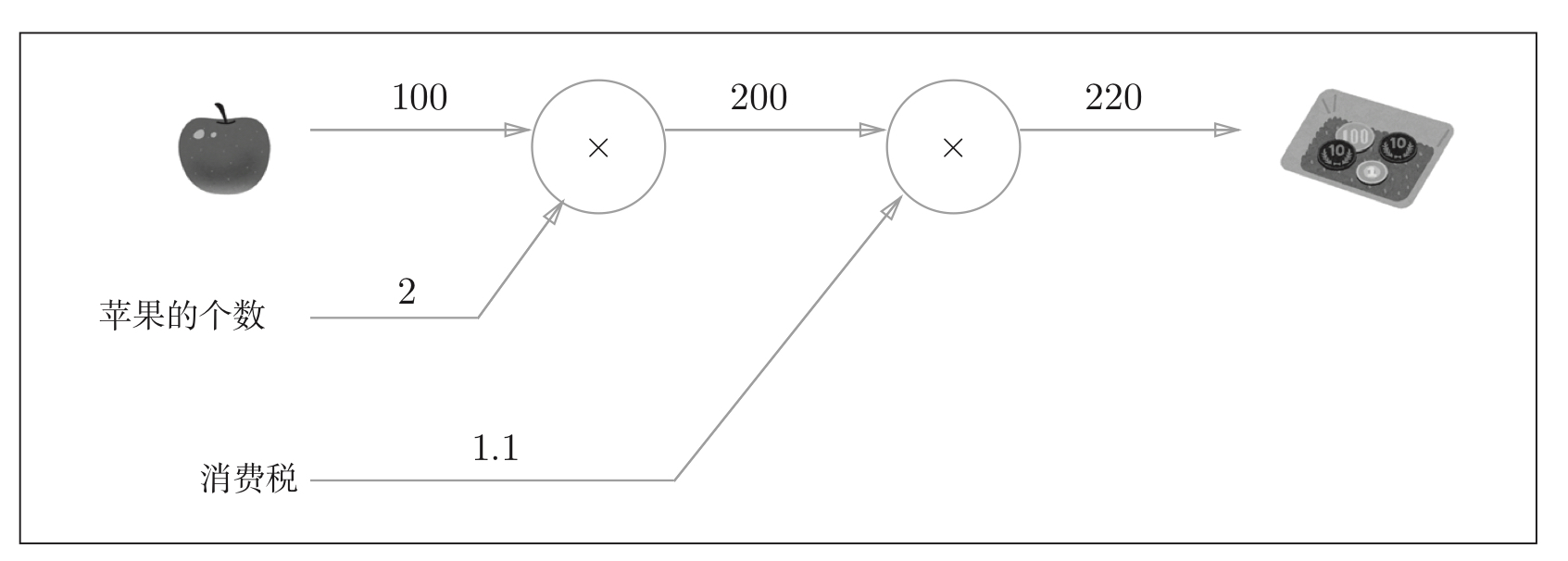
Figure 1: solve problem 1 based on the calculation diagram: the number of apples and consumption tax are marked externally as variables
Question 2: Xiao Ming bought two 100 yen apples and three 150 yen oranges in the supermarket. The consumption tax is 10%. Calculate the amount Xiao Ming paid.

Figure 2: solve problem 2 based on the calculation diagram: the number of apples and oranges and consumption tax are marked externally as variables
Based on the above solution, the calculation flow of the calculation diagram can be obtained:
- Build calculation diagram
- On the calculation chart, calculate from left to right
Forward propagation: calculation from left to right is called forward propagation
Back propagation: it is also possible to calculate from right to left, which is called back propagation and plays an important role in calculating derivatives
5.1.2 local calculation
For example, if you buy two apples and other things in the supermarket, you can draw the following calculation diagram:

Figure 3: bought two apples and other things
It can be seen from the above figure that the calculation diagram can focus on local calculation. No matter how complex the global calculation is, all the steps need to do is the local calculation of the object node.
5.1.3 why use calculation chart to solve problems
Through the calculation diagram, the gradient can be calculated efficiently using back propagation.
Example: in solving problem 1, the derivative of the price of the total amount paid.
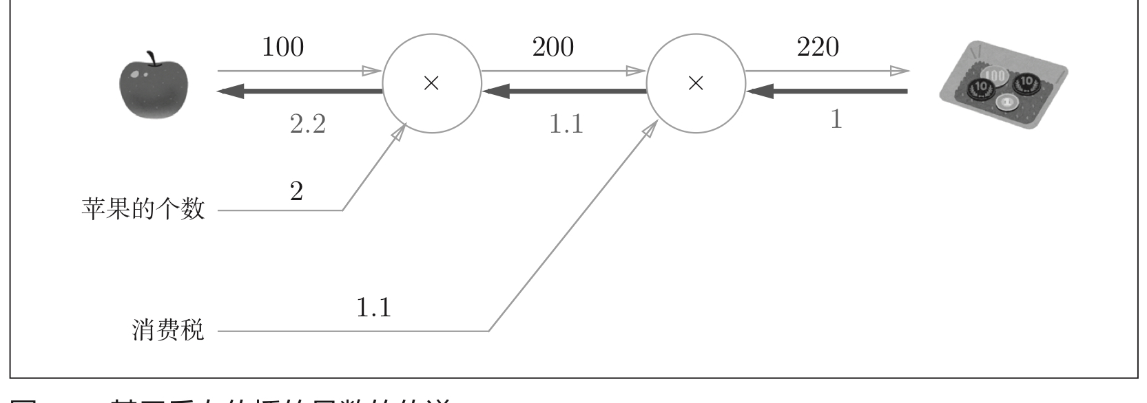
Figure 4: I bought two apples, and the derivative of consumption amount to apple price
According to the above figure, the derivative of consumption amount to apple price is 2.2, that is, for every unit of apple price change, the consumption amount will increase by 2.2 units. During the calculation of apple price derivative, other derivatives can also be solved, and the derivative can be shared, such as the gradient between the total amount of final consumption and the total amount excluding consumption tax.
5.2 chain rule
Chain rule: the core of back propagation.
5.2.1 back propagation of calculation diagram

Figure 5: back propagation of calculation diagram
5.2.2 what is the chain rule
The chain rule is about the properties of the derivatives of composite functions:
- If a function is represented by a composite function, the derivative of the composite function can be expressed by the product of the derivatives of each function constituting the composite function.

Figure 6: steps of derivation of composite function
5.2.3 chain rule and calculation diagram
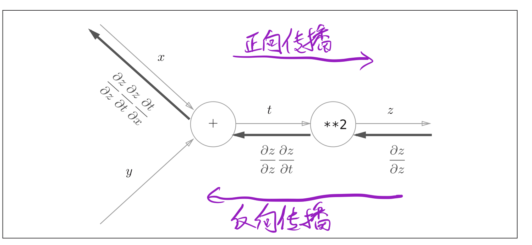
Figure 7: calculation diagram to solve the gradient of composite function

Figure 8: calculation diagram to solve the gradient of composite function (bring in specific data)
Through the above two figures, we can understand the process of calculating the gradient information through the chain rule.
5.3 back propagation (based on calculation diagram)
Back propagation is based on the chain rule. This section will introduce the structure of back propagation by taking operations such as + and x as examples
5.3.1 back propagation of addition node
Take z = x + y, z = x + YZ = x + y as an example.
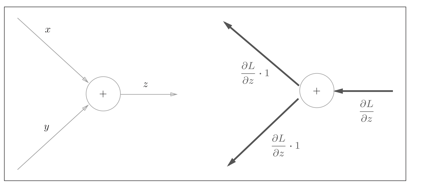
Figure 9: the back propagation of the addition node is shown in the figure above: the graph of coordinates is the forward propagation, and the right is the back propagation. For the back propagation of the addition node, the downstream gradient value is equal to the upstream gradient value.
Back propagation of local calculation addition node:
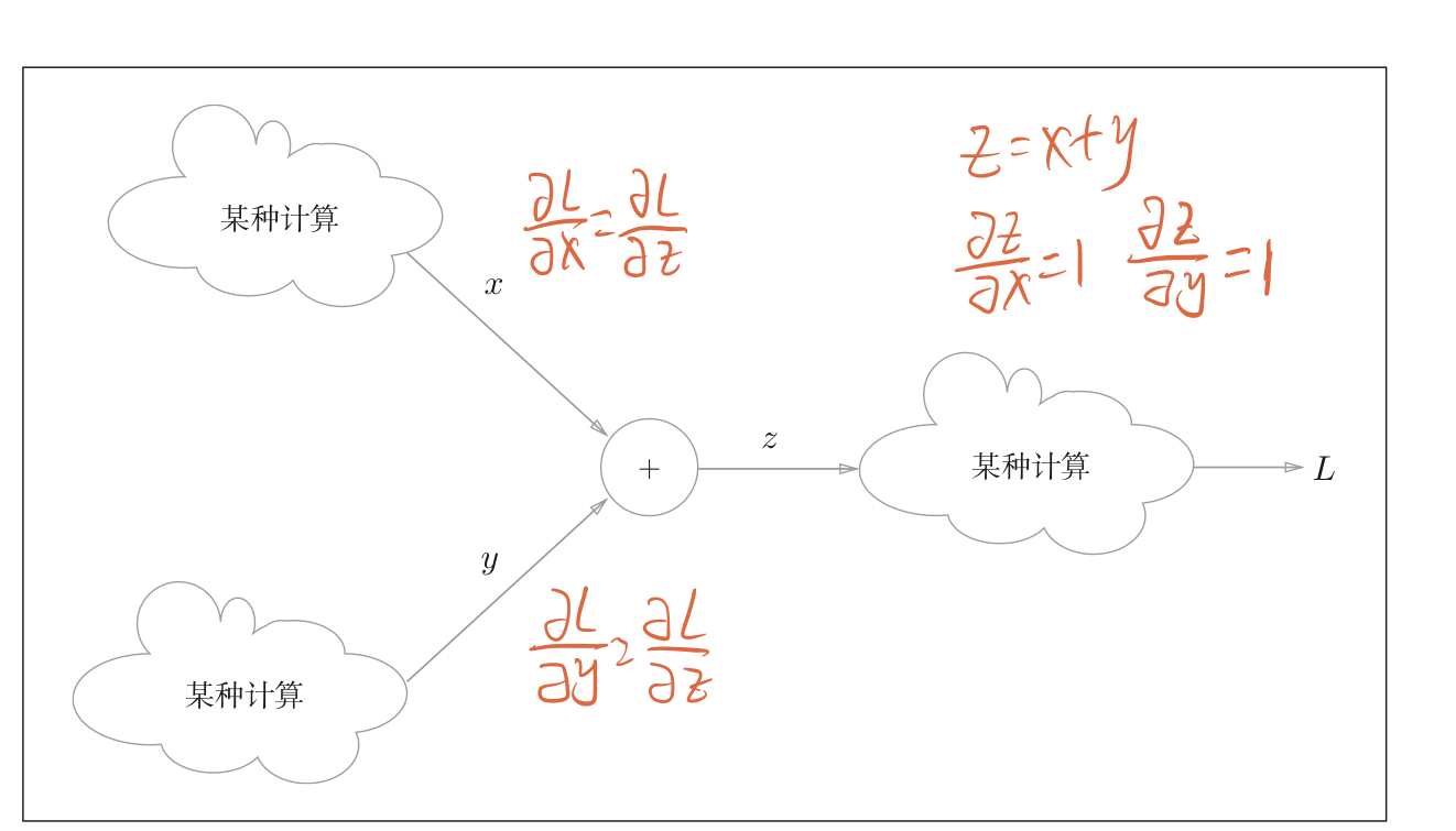
Figure 10: backpropagation of locally calculated addition nodes for a large network, the backpropagation result of an addition node at a certain place is still valid.
A practical example: 10 + 5 = 15, 10 + 5 = 1510 + 5 = 15. During back propagation, the gradient value transmitted from the upstream is 1.3

Figure 11: example of backpropagation of locally calculated addition nodes
5.3.2 back propagation of multiplication node
Take z = x * y, z = x * YZ = x * y as an example.

Figure 12: back propagation of multiplication node is shown in the figure above: the figure on the left is forward propagation and the figure on the right is back propagation
Practical examples:

Figure 13: the gradient value from upstream is 1.3
- The back propagation of multiplication will be multiplied by the inversion value of the input signal, that is, the derivative of 10 should be 1.35 = 6.5; The derivative of 5 should be 1.310 = 13;
- When realizing the back propagation of multiplication node, the input signal of forward propagation should be saved
Examples of hand training:
After understanding the back propagation of addition node and multiplication node, you can try the following questions and fill in the results:

Figure 14: inspection problems
5.4 code implementation of back propagation (based on calculation diagram)
It can be seen from the above that there are two cases to solve the gradient through the calculation graph, multiplication node and addition node. Here, we define two layers: multiplication layer and addition layer to realize the derivation of the problem in these two cases. Many problems are the combination of addition layer and multiplication layer.
5.4.1 implementation of multiplication layer
class MulLayer:
    def __init__(self):
        self.x=None
        self.y=None

    #Forward propagation
    def forward(self,x,y):
        self.x=x
        self.y=y
        out=x *y

        return out
    def backward(self,dout):#dout is the derivative passed down from the upper layer
        #Flip x and y
        dx=dout * self.y
        dy=dout * self.x

        return dx,dy
5.4.2 implementation of addition layer
class Addlayer:
    def __init__(self):
       pass  #No need to pass parameters

    #Forward forward
    def forward(self,x,y):
        out=x+y
        return out

    #backward
    def backward(self,out):
        dx=dout
        dy=dout
        return dx,dy
5.4.3 solution to problem 1
Repeat question 1: * Xiao Ming bought two apples of 100 yen each in the supermarket, and the consumption tax is 10%. Calculate the amount Xiao Ming paid, calculate the unit price of the payment amount to the apple, the number of apples, and the gradient of the tax rate?
#Two of Apple's back propagation errors:
#Implementation of deep learning simple layer (multiplication layer and addition layer)
class MulLayer:
    def __init__(self):
        self.x=None
        self.y=None

    #Forward propagation
    def forward(self,x,y):
        self.x=x
        self.y=y
        out=x *y

        return out
    def backward(self,dout):#dout is the derivative passed down from the upper layer
        #Flip x and y
        dx=dout * self.y
        dy=dout * self.x

        return dx,dy
class Addlayer:
    def __init__(self):
       pass  #No need to pass parameters

    #Forward forward
    def forward(self,x,y):
        out=x+y
        return out

    #backward
    def backward(self,out):
        dx=dout
        dy=dout
        return dx,dy

#Define initial value
apple=100
appel_num=2
tax=1.1

#Definition layer
mul_apple_layer=MulLayer()
mul_tax_layer=MulLayer()

#forward
apple_price=mul_apple_layer.forward(apple,appel_num)
price=mul_tax_layer.forward(apple_price,tax)
print('price=','%.1f'%price)

# backward
dprice = 1
dapple_price, dtax = mul_tax_layer.backward(dprice)
dapple, dapple_num = mul_apple_layer.backward(dapple_price)

#Output results
print('dapple=',dapple)
print('dapple_num=',int(dapple_num))
print('dtax=',dtax)
5.4.3 solution to problem 2
Repeat question 2: * Xiao Ming bought two apples of 100 yen each and three oranges of 150 yen each in the supermarket. The consumption tax is 10%. Calculate the amount Xiao Ming paid, the unit price of the payment amount to the apple, the quantity of apples, the unit price of oranges, the quantity of oranges, and the gradient of tax rate?
#Error back propagation for purchasing two apples and three oranges (including error back propagation for addition and multiplication):
#Implementation of deep learning simple layer (multiplication layer and addition layer)
class MulLayer:
    def __init__(self):
        self.x=None
        self.y=None

    #Forward propagation
    def forward(self,x,y):
        self.x=x
        self.y=y
        out=x *y

        return out
    def backward(self,dout):#dout is the derivative passed down from the upper layer
        #Flip x and y
        dx=dout * self.y
        dy=dout * self.x

        return dx,dy
class AddLayer:
    def __init__(self):
       pass  #No need to pass parameters

    #Forward forward
    def forward(self,x,y):
        out=x+y
        return out

    #backward
    def backward(self,dout):
        dx=dout
        dy=dout
        return dx,dy

#Define initial value
apple=100
orange=150
appel_num=2
orange_num=3
tax=1.1

#Definition layer
mul_apple_layer=MulLayer()
mul_orange_layer=MulLayer()
mul_tax_layer=MulLayer()
add_orange_apple_layer=AddLayer()

#forward
apple_price=mul_apple_layer.forward(apple,appel_num)
orange_price=mul_orange_layer.forward(orange,orange_num)
sum_price=add_orange_apple_layer.forward(apple_price,orange_price)
price=mul_tax_layer.forward(sum_price,tax)
print('sumprice=','%.1f'%price)

# backward
dprice = 1
dsum_price, dtax = mul_tax_layer.backward(dprice)
dapple_price,dorange_price=add_orange_apple_layer.backward(dsum_price)
dorange,dorange_num=mul_orange_layer.backward(dorange_price)
dapple,dapple_num=mul_apple_layer.backward(dapple_price)

#Output results
print('dapple=','%.1f'%dapple,'dapple_num=',int(dapple_num))
print('dorange=','%.1f'%dorange,'dorange_num=',int(dorange_num))

print('dtax=',dtax,'dapple_price=',dapple_price)
5.5 implementation of activation function layer (based on calculation diagram)
Applying the thinking of computational graph to neural network, we define the implementation of neural network layer as a class. The activation function layer is realized through addition layer and multiplication layer. Activation functions include: ReLU layer and Sigmoid layer
5.5.1 ReLU layer
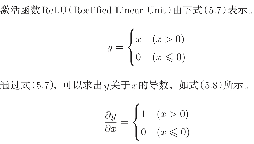
Figure 15: function expression and gradient expression of activation function ReLU Figure 16: calculation diagram of ReLU layer
Implementation code:
class ReLU:
    def __init__(self):
        self.mask=None

    #Forward propagation
    def forward(self,x):
        self.mask=(x<=0)  #mask a logical array in which the values of x < = are True
        out=x.copy()      #out equals x
        out[self.mask]=0  #Set the value of True in the mask to 0
                          #It is equivalent to completing the function of ReLU, which is 0 when it is less than or equal to 0; When it is greater than 0, keep the original value
        return out
    #Back propagation
    def backward(self,dout):
        dout[mask]=0
        df=dout
        return df
5.5.2 Sigmoid layer
According to the definition, the function expression of Sigmoid is:
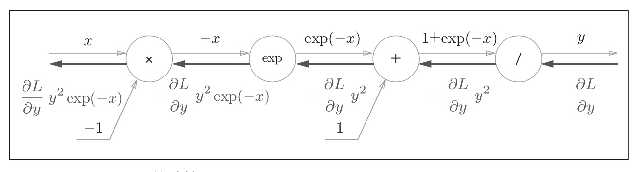
Figure 17: calculation diagram of activation function Sigmoid Figure 18: simplified calculation diagram of activation function Sigmoid
Code implementation:
class Sigmoid():
    def __init__(self):
        self.out=None

    def forward(self,x):
        out=1/(1+np.exp(-x))
        self.out=out
        return out

    def backward(self,dout):
        return dout*self.out*(1.0-self.out)
5.5.3 Affine layer
In the forward propagation of neural network, it is necessary to calculate the sum of weighted signals. Here, the Affine layer is used to define this operation.
Function expression of affinity layer (X, W and B are matrices): y = X * W+B y = XW + by * = x * W+B

Figure 19: calculation diagram of affinity layer of batch version
Code implementation:
class Affine():                     #Change all the important parameters into instance variables
    def __init__(self,W,b):
        self.W=W
        self.b=b
        self.x=None
        self.dW=None
        self.db=None

    def forward(self,x):
        self.x=x
        out=self.x*self.W+b
        self.out=out
        return out

    def backward(self,dout):
        dx=np.dot(dout,self.W.T)
        dW=np.dot(self.x.T,dout)
        db=np.sum(dout,axis=0)

        return dx
5.5.4 softmax with loss layer
If the neural network is used for classification, the last layer is the Softmax layer. Due to the need for training data, the last layer in the training network also needs a loss function layer to evaluate the advantages and disadvantages of the selected parameters.

Figure 20: calculation diagram of softmax with loss layer

Figure 21: simplified version - calculation diagram of softmax with loss layer
In Figure 21, the softmax layer and cross entry error layer are encapsulated during forward propagation, which can be seen more clearly.
Code implementation:
class SoftmaxWithLoss():
    def __init__(slef):
        self.loss=None   #loss
        self.y=None      #Output of softmax
        self.t=None      #one hot vector

    def forward(self,x,t):
        self.t=t
        self.y=softmax(x)
        self.loss=cross_entropy_error(self.y,self.t)  #Use the softmax and cross defined above_ entropy_ Error calculate the error value

        return self.loss

    def backward(self,dout=1):
        batch.size=self.t.shape[0]
        dx=(self.y-self.t)/batch_size   #The reason why the gradient is divided by the batch: the previous error is a batch
                                        #      The sum of the mean square error, divided by batch -- size, is
                                        #      What is passed to the previous layer is the error of a single data
                                        #      The gradient formula here is derived
        return dx
5.6 error Back propagation (code implementation based on calculation diagram)
There are two ways to realize the code in this chapter:
- The first one: directly modify the sub function of solving the gradient, and other parts are the same as in the previous chapter.
- The second is to modify the class of two-layer neural network and divide the neural network into layers.
Both methods have advantages and disadvantages:
- In the first method, the gradient function is modified directly. The operation is relatively simple, but the content is relatively complex. If the number of layers of the network is deepened, it will be difficult to write the corresponding gradient function.
- The second method has many changes, but the hierarchical structure is simple, which is very suitable for expanding to a deeper network structure.
5.6.1 implementation of method 1
This method only changes the sub function of solving the gradient. Here, a two-layer network is taken as an example to list the sub functions before and after modification.
(before modification) gradient calculation by numerical differentiation method:
 def numerical_gradient(self,x,t):
        loss_W=lambda W:self.loss(x,t)      #I don't understand. What do you mean

        grads={}  #Define the gradient information of parameters and access the gradient information value of weight parameters

        #The gradient information values of the four weight parameters are obtained and stored in grad
        grads['W1']=numerical_gradient(loss_W,self.params['W1'])
        grads['b1']=numerical_gradient(loss_W,self.params['b1'])
        grads['W2']=numerical_gradient(loss_W,self.params['W2'])
        grads['b2']=numerical_gradient(loss_W,self.params['b2'])

        return grads
(modified) error reverse broadcast gradient:
def gradient(self, x, t):
        W1, W2 = self.params['W1'], self.params['W2']
        b1, b2 = self.params['b1'], self.params['b2']

        grads = {}

        batch_num = x.shape[0]

        # forward
        a1 = np.dot(x, W1) + b1
        z1 = sigmoid(a1)
        a2 = np.dot(z1, W2) + b2
        y = softmax(a2)              #Define by yourself, you can stack multiple layers

        # backward
        dy = (y - t) / batch_num
        grads['W2'] = np.dot(z1.T, dy)
        grads['b2'] = np.sum(dy, axis=0)

        da1 = np.dot(dy, W2.T)
        dz1 = sigmoid_grad(a1) * da1
        grads['W1'] = np.dot(x.T, dz1)
        grads['b1'] = np.sum(dz1, axis=0)

        return grads
5.6.2 implementation of method 2
For two layers neural network Has been greatly modified. Many types of activation function layers are defined. The back prediction is expressed by forward propagation, and the gradient is expressed by error back propagation results. The direct construction of layers is clear at a glance, which is convenient for the amplification of the back structure.
For the last blog (numerical differentiation method) minist neural network learning The code for realizing neural network in. There are 5 modifications here:
- To write an additional file layer for calling the activation function layer to facilitate the call of neural network classes.
- In__ init__ () subfunction defines the layers used in the network
- In the sub function predict(), the forward propagation value is directly obtained for each layer at a time, instead of writing the results one by one.
- In the loss() subfunction, the loss function no longer uses cross_ entropy_ The error () function is obtained, but it is directly solved with the SoftmaxWithLoss layer.
- The last one is to solve the change of gradient function, which changes greatly here.
5.6.3 implementation code of method 2
There are three main files to implement this file:
- TLN_main.py: the main function is the same as that of the previous blog, with no change
- TLN_function.py: store some activation functions without change
- Layer.py: a new file is added to store the functions of the active function layer (based on the calculation diagram)
- two_layer_net1.py: there are many changes. The changes have just been described (they are also marked in the following code)
5.6.3.1 document I: TLN_main.py
File 1: TLN_main.py
'''#Implementation of ini batch algorithm ''
#Call of related Library
import time
import numpy as np
import matplotlib.pyplot as plt
import sys,os
sys.path.append(os.pardir)   #The first two lines of code are purely to call functions in documents across folders
from dataset.mnist import load_mnist        #Call the function that loads the mnist dataset
from two_layer_net1 import TwoLayerNet       #Call the class composed of edited two-layer neural network
#from two_layer_net import TwoLayerNet


#Data acquisition of handwritten dataset mnist
(x_train,t_train),(x_test,t_test)=load_mnist(flatten=True,normalize=True,one_hot_label=True)
#load_mnist reads the data set in the form of (training picture, training label), (test picture, test label)
#Normalize: whether to normalize the input picture to a value of 0.0-1.0. There is no normalization here, and the picture pixels are still 0-255
#flatten: whether to expand the input image (into a one-dimensional array). Here, it is displayed in a one-dimensional array
#one_hot_label: only arrays with correct labels of 1 and other 0, such as [0,0,0,1,0,0]. If False, only labels with correct solutions such as 2,7 will be saved


#Average number of repetitions per epoch


#Definition of super parameters
iters_num=10000
train_size=x_train.shape[0]   #Size of total training set
batch_size=100                #mini_batch size
learning_rate=0.5                #The learning rate is also equivalent to the step size

network= TwoLayerNet(input_size=784,hidden_size=100,output_size=10)
#Define the basic parameters of the two-layer neural network:
#Neural network: two layers, 784 inputs, 50 hidden neurons and 10 outputs.

#Define some matrices to calculate the loss function and accuracy value
train_loss_list=[]  #Training loss function
train_acc_list=[]   #Accuracy of training data
test_acc_list=[]    #Accuracy of test data
iter_per_epoch=max(train_size/batch_size,1)


#Main function
start = time.clock()    #Timing start

for i in range(iters_num):

    #Get random mini batch
    batch_mask=np.random.choice(train_size,batch_size)  #Select batch from the total number of training sets_ Size is a random number without repetition
    x_batch=x_train[batch_mask]
    t_batch=t_train[batch_mask]

    #Calculated gradient
    #grad=network.numerical_gradient(x_batch,t_batch)
    #Using the error back propagation method:
    grad=network.gradient(x_batch,t_batch)

    #Update parameters
    for key in ('W1','b1','W2','b2'):
        network.params[key] -= learning_rate*grad[key]

    #Record the learning process
    loss=network.loss(x_batch,t_batch)
    train_loss_list.append(loss)         #Do not understand the meaning of the code


    #After every epoch (parameter update), the recognition accuracy is calculated for all training data and test data
    if i % iter_per_epoch==0:
        #Record of training data and test data
        train_acc=network.accuracy(x_train,t_train)
        test_acc=network.accuracy(x_test,t_test)

        train_acc_list.append(train_acc)
        test_acc_list.append(test_acc)

       # print('train_acc,test_acc| '+str(train_acc)+' , '+test_acc)
        print('train_acc,test_acc|', train_acc,',',test_acc)

#Add a timing function
end = time.clock()           #End of timing
print ('Running time:',str(end-start))   #Displays the elapsed time

#Draw graphics

x = np.arange(len(train_acc_list))                            #Draw the three main lines of the image, variables and dependent variables
plt.plot(x, train_acc_list, label='train acc', marker='o')
plt.plot(x, test_acc_list, label='test acc', marker='x',linestyle='--')

plt.xlabel("epochs")            #A label that displays the abscissa and ordinate
plt.ylabel("accuracy")
plt.ylim(0, 1.0)
plt.legend(loc='lower right')  #The legend is displayed in the lower right corner

plt.savefig('./test2.jpg')     #Save the displayed picture
plt.show()
5.6.3.2 document II: TLN_function.py
Document 2: TLN_function.py
#Subfunctions in TwoLayerNet
import numpy as np
#Find gradient function
def numerical_gradient(f, x):
    h = 1e-4 # 0.0001
    grad = np.zeros_like(x)

    it = np.nditer(x, flags=['multi_index'], op_flags=['readwrite'])
    while not it.finished:
        idx = it.multi_index
        tmp_val = x[idx]
        x[idx] = float(tmp_val) + h
        fxh1 = f(x) # f(x+h)

        x[idx] = tmp_val - h
        fxh2 = f(x) # f(x-h)
        grad[idx] = (fxh1 - fxh2) / (2*h)

        x[idx] = tmp_val # Restore value
        it.iternext()

    return grad

#Activation function (used between layers)
def sigmoid(x):
    return 1 / (1 + np.exp(-x))

#Activation function (used by output layer)
def softmax(x):
    if x.ndim == 2:
        x = x.T
        x = x - np.max(x, axis=0)
        y = np.exp(x) / np.sum(np.exp(x), axis=0)
        return y.T

    x = x - np.max(x) # Spillover Countermeasures
    return np.exp(x) / np.sum(np.exp(x))

#Calculation of loss function
def cross_entropy_error(y, t):
    if y.ndim == 1:
        t = t.reshape(1, t.size)
        y = y.reshape(1, y.size)

    # When the supervision data is one hot vector, it is converted to the index of correctly unlabeled
    if t.size == y.size:
        t = t.argmax(axis=1)

    batch_size = y.shape[0]
    return -np.sum(np.log(y[np.arange(batch_size), t] + 1e-7)) / batch_size

#Subfunction to be used in error back propagation algorithm
def sigmoid_grad(x):
    return (1.0 - sigmoid(x)) * sigmoid(x)
5.6.3.3 document III: layer py
File 3: layer py
#Implementation of activation layer, four (ReLU, Sigmoid, affiliate, softmaxwithloss)

import numpy as np
from TLN_function import *


class ReLU:
    def __init__(self):
        self.mask=None

    #Forward propagation
    def forward(self,x):
        self.mask=(x<=0)  #mask a logical array in which the values of x < = are True
        out=x.copy()      #out equals x
        out[self.mask]=0  #Set the value of True in the mask to 0
                          #It is equivalent to completing the function of ReLU, which is 0 when it is less than or equal to 0; When it is greater than 0, keep the original value
        return out
    #Back propagation
    def backward(self,dout):
        dout[self.mask]=0
        df=dout
        return df

class Sigmoid():
    def __init__(self):
        self.out=None

    def forward(self,x):
        out=1 / (1 + np.exp(-x))
        self.out=out
        return out

    def backward(self,dout):
        return dout*(1.0-self.out)*self.out

class Affine():                     #Change all the important parameters into instance variables
    def __init__(self,W,b):
        self.W=W
        self.b=b
        self.x=None
        self.original_x_shapr=None             ####Define the shape of x
        self.dW=None
        self.db=None

    def forward(self,x):
        self.original_x_shape =x.shape        #####Save the shape of x
        x=x.reshape(x.shape[0],-1)            #####Restore the shape of x
        self.x=x
        out=np.dot(x,self.W)+self.b

        return out

    def backward(self,dout):
        dx=np.dot(dout,self.W.T)
        self.dW=np.dot(self.x.T,dout)
        self.db=np.sum(dout,axis=0)

        dx=dx.reshape(*self.original_x_shape)   #Restore the shape of the input data (corresponding tensor)

        return dx

class SoftmaxWithLoss():
    def __init__(self):
        self.loss=None   #loss
        self.y=None      #Output of softmax
        self.t=None      #one hot vector

    def forward(self,x,t):
        self.t=t
        self.y=softmax(x)
        self.loss=cross_entropy_error(self.y,self.t)  #Use the softmax and cross defined above_ entropy_ Error calculate the error value

        return self.loss

    def backward(self,dout=1):
        batch_size=self.t.shape[0]
        if self.t.size ==self.y.size:    ####The supervision data is one-hot-vector case (a judgment is added to determine whether it is one-hot-vector case)
            dx=(self.y-self.t)/batch_size   #The reason why the gradient is divided by the batch: the previous error is a batch
                                        #      The sum of the mean square error, divided by batch -- size, is
                                        #      What is passed to the previous layer is the error of a single data
                                        #      The gradient formula here is derived
        else:                                      ###
            dx=self.y.copy()                        ###
            dx[np.arange(batch_size),self.t] -= 1
            dx= dx/batch_size
        return dx
5.6.3.4 document IV: two_layer_net1.py
Document 4: two_layer_net1.py
#Two layer network structure using error back propagation

#Import of libraries and functions

import sys,os
import numpy as np
sys.path.append(os.pardir)          #The first two lines of code are purely to call functions in documents across folders
from TLN_function import *          #Call TLN_ All sub functions in function file
from Layer import *                 #call Layer All subfunctions in the file                 newly added#######
from collections import OrderedDict  #Calling from the internal library OrderdDict This ordered dictionary      newly added#######


class TwoLayerNet:


    def __init__(self,input_size,hidden_size,output_size,weight_init_std=0.01):

        #Initialize the weight and define several instance variables (that is, local variables in the class)
        self.params={}   #Initialize the instance variable params, which contains four variables: W1, W2, B1 and B2

        #W1 and W2 are initialized with random numbers conforming to Gaussian distribution
        self.params['W1']=weight_init_std*np.random.randn(input_size,hidden_size)
        self.params['W2']=weight_init_std*np.random.randn(hidden_size, output_size)
        #b1 and b2 are initialized with 0
        self.params['b1']=np.zeros(hidden_size)    #The initial values are all set to 0
        self.params['b2']=np.zeros(output_size)    #The initial values are all set to 0

        #Generation layer                                                               newly added#######
        self.layers=OrderedDict()

        self.layers['Affinel'] = Affine(self.params['W1'],self.params['b1'])
        self.layers['Relu1'] = ReLU()
        self.layers['Affine2'] = Affine(self.params['W2'],self.params['b2'])

        self.lastLayer = SoftmaxWithLoss()


    def predict(self,x):                                                     #modify#######
        for layer in self.layers.values():       #The value function operates on the dictionary variable to obtain the value of the dictionary variable
            x=layer.forward(x)

        return x
    '''
    def predict(self,x):

        #Assignment variable
        W1,W2=self.params['W1'],self.params['W2']
        b1,b2=self.params['b1'],self.params['b2']

        #Forward propagation algorithm for two-layer networks
        a1=np.dot(x,W1)+b1
        z1=sigmoid(a1)
        a2=np.dot(z1,W2)+b2
        y=softmax(a2)

        return y
    '''

    #x: Image data; t: Untag correctly
    #Loss function (cross entropy error function u, calculate the loss value)
    def loss(self,x,t):                                                       #modify
        y=self.predict(x)
        #loss_x=cross_entropy_error(y,t)                                     #Modification, two things mean the same thing
        loss_x=self.lastLayer.forward(y,t)

        return loss_x

    #Calculation accuracy function
    def accuracy(self,x,t):
        y=self.predict(x)
        y=np.argmax(y,axis=1)   #Find the maximum value in each column in y
        t=np.argmax(t,axis=1)   #Find the maximum value in each column in t

        accuracy=np.sum(y==t)/float(x.shape[0])   #Cast type
        return accuracy

    #x: Image data; t: Untag correctly
    #Calculate the gradient of the weight parameter


    #Two algorithms for solving gradient
    #Solving the gradient value of weight parameters by negative gradient method
    def numerical_gradient(self,x,t):
        loss_W=lambda W:self.loss(x,t)      #I don't understand. What do you mean

        grads={}  #Define the gradient information of parameters and access the gradient information value of weight parameters

        #The gradient information values of the four weight parameters are obtained and stored in grad
        grads['W1']=numerical_gradient(loss_W,self.params['W1'])
        grads['b1']=numerical_gradient(loss_W,self.params['b1'])
        grads['W2']=numerical_gradient(loss_W,self.params['W2'])
        grads['b2']=numerical_gradient(loss_W,self.params['b2'])

        return grads

    #Solving gradient value by error back propagation method
    def gradient(self, x, t):                                              #Major modifications

        #forward
        self.loss(x,t)

        #backward
        dout=1
        dout=self.lastLayer.backward(dout)

        layers=list(self.layers.values())
        layers.reverse()                                #Reverse this dictionary vector
        for layer in layers:
            dout=layer.backward(dout)

        #set up
        grads={}  #Define the gradient information of parameters and access the gradient information value of weight parameters

        #The gradient information values of the four weight parameters are obtained and stored in grad
        #The updated values are stored in a matrix
        grads['W1']=self.layers['Affinel'].dW
        grads['b1']=self.layers['Affinel'].db
        grads['W2']=self.layers['Affine2'].dW
        grads['b2']=self.layers['Affine2'].db

        return grads
5.6.3.5. Operation results
>>>start = time.clock()    #Timing start
>>>train_acc,test_acc| 0.16121666666666667 , 0.1615
>>>train_acc,test_acc| 0.9480833333333333 , 0.9461
>>>train_acc,test_acc| 0.9716 , 0.9669
>>>train_acc,test_acc| 0.9767333333333333 , 0.972
>>>,test_acc| 0.9813333333333333 , 0.9727
>>>train_acc,test_acc| 0.9871333333333333 , 0.973
>>>train_acc,test_acc| 0.9903833333333333 , 0.9748
>>>train_acc,test_acc| 0.9923666666666666 , 0.9782
>>>,test_acc| 0.9934833333333334 , 0.9767
>>>train_acc,test_acc| 0.99525 , 0.9784
>>>train_acc,test_acc| 0.9958666666666667 , 0.978
>>>train_acc,test_acc| 0.9983833333333333 , 0.9794
>>>Running time: 44.66675650000002   #Total time
Picture output:
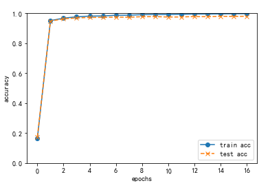
Figure 1: output pictures (change of accuracy rate) the accuracy of test set and training set changes little, indicating that the training model has not been fitted and the effect is relatively good.
'Affine2'].dW
grads['b2']=self.layers['Affine2'].db
return grads
##### 5.6.3.5.  Operation results

```python
>>>start = time.clock()    #Timing start
>>>train_acc,test_acc| 0.16121666666666667 , 0.1615
>>>train_acc,test_acc| 0.9480833333333333 , 0.9461
>>>train_acc,test_acc| 0.9716 , 0.9669
>>>train_acc,test_acc| 0.9767333333333333 , 0.972
>>>,test_acc| 0.9813333333333333 , 0.9727
>>>train_acc,test_acc| 0.9871333333333333 , 0.973
>>>train_acc,test_acc| 0.9903833333333333 , 0.9748
>>>train_acc,test_acc| 0.9923666666666666 , 0.9782
>>>,test_acc| 0.9934833333333334 , 0.9767
>>>train_acc,test_acc| 0.99525 , 0.9784
>>>train_acc,test_acc| 0.9958666666666667 , 0.978
>>>train_acc,test_acc| 0.9983833333333333 , 0.9794
>>>Running time: 44.66675650000002   #Total time
Picture output:
Figure 1: output pictures (change of accuracy rate) the accuracy of test set and training set changes little, indicating that the training model has not been fitted and the effect is relatively good.