Chapter IV basis of pandas statistical analysis

4.1 read / write data from different data sources

4.1.1 read / write database data

1. Database data reading

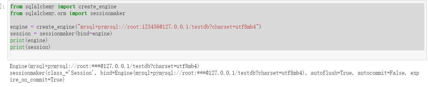
from sqlalchemy import create_engine
from sqlalchemy.orm import sessionmaker

engine = create_engine("mysql+pymysql://root:123456@127.0.0.1/testdb?charset=utf8mb4")
session = sessionmaker(bind=engine)
print(engine)
print(session)

Operation results:

#Using read_sql_table,read_sql_query,read_sql function reads database data
import pandas as pd
formlist=pd.read_sql_query('show tables',con=engine)
print('testdb The list of database data tables is:','\n',formlist)

Operation results:

# Using read_sql_table read order details table
detail1=pd.read_sql_table('meal_order_detail1',con=engine)
print('use read_sql_table The length of reading order details table is',len(detail1))
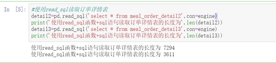
#Using read_sql read order details table
detail2=pd.read_sql('select * from meal_order_detail2',con=engine)
print('use read_sql function+sql The length of the statement to read the order details table is',len(detail2))
detail3=pd.read_sql('select * from meal_order_detail3',con=engine)
print('use read_sql function+sql The length of the statement to read the order details table is',len(detail3))

Operation results:

2. Database data storage

be careful

Before doing this, remember to directly change the database code to utf8mb4_general_ci, which is also used when connecting to the database in Python code
charset = "utf8mb4", and set the code of test1 table to be consistent. Enter the corresponding database on the cmd side and set alter table test1 convert to character set utf8mb4;

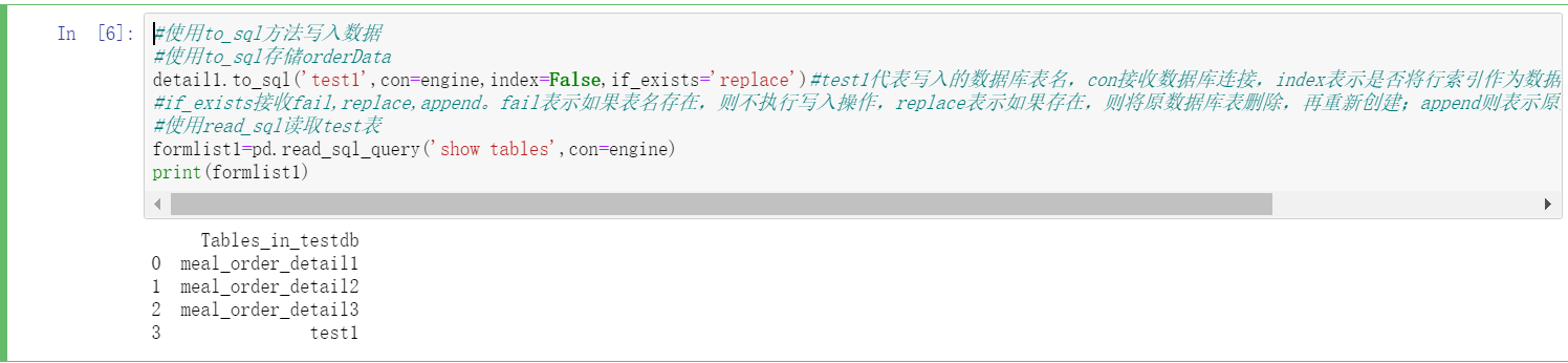
#Use to_sql method writes data
#Use to_sql store orderData
detail1.to_sql('test1',con=engine,index=False,if_exists='replace')#test1 represents the name of the written database table, con receives the database connection, and index indicates whether to transfer the row index into the database as data,
#if_exists receives fail,replace,append. Fail means that if the table name exists, the write operation will not be performed. Replace means that if it exists, the original database table will be deleted and recreated; Append means to append data based on the original database table. The default is fail
#Using read_sql read test table
formlist1=pd.read_sql_query('show tables',con=engine)
print(formlist1)

Operation results:

4.1.2 reading / writing text files

1. Text file reading

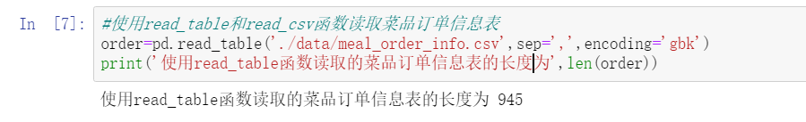
#Using read_table and read_csv function reads dish order information table
order=pd.read_table('./data/meal_order_info.csv',sep=',',encoding='gbk')
print('use read_table The length of the dish order information table read by the function is',len(order))

Operation results:

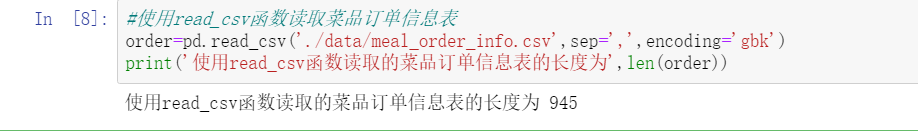
#Using read_csv function reads dish order information table
order=pd.read_csv('./data/meal_order_info.csv',sep=',',encoding='gbk')
print('use read_csv The length of the dish order information table read by the function is',len(order))

Operation results:

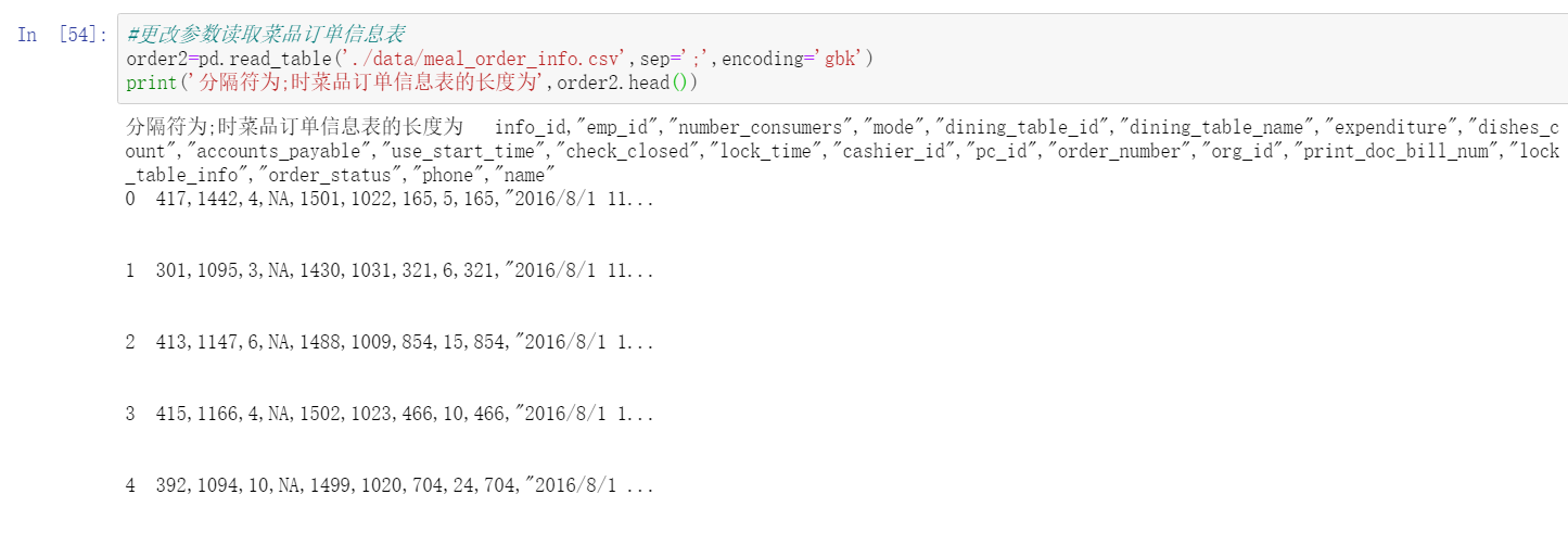
#Change the parameters to read the dish order information table
order2=pd.read_table('./data/meal_order_info.csv',sep=';',encoding='gbk')
print('Separator is;The length of the dish order information table is',order2)

Operation results:

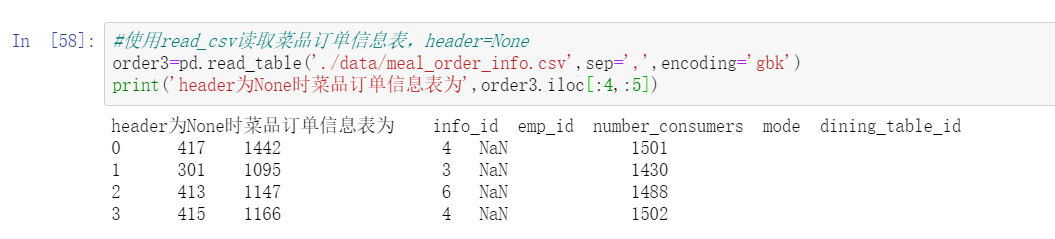
#Using read_csv reads the dish order information table, header=None
order3=pd.read_table('./data/meal_order_info.csv',sep=',',encoding='gbk')
print('header by None The dish order information table is',order3.iloc[:4,:5])

Operation results:

4.1.3 reading / writing Excel files

1. Excel file reading

#Using read_ Reading dish order information with Excel function
user=pd.read_excel('./data/users.xlsx')#read file
print('Length of customer information table:',len(user))

2. Excel file storage

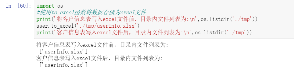
import os
#Use to_excel functions store data as excel files
print('Write customer information table to excel Before the file, the list of files in the directory is:\n',os.listdir('./tmp'))
user.to_excel('./tmp/userInfo.xlsx')
print('Customer information table writing excel After the file, the list of files in the directory is:\n',os.listdir('./tmp'))

Operation results:

4.1.4 task realization

1. Read order details database data

#Read order details table
from sqlalchemy import create_engine
import pandas as pd
engine = create_engine("mysql+pymysql://root:123456@127.0.0.1/testdb?charset=utf8mb4")
session = sessionmaker(bind=engine)
detail1=pd.read_sql_table('meal_order_detail1',con=engine)
print('use read_sql_table The length of reading order details Table 1 is',len(detail1))
detail2=pd.read_sql_table('meal_order_detail2',con=engine)
print('use read_sql_table The length of reading order details Table 2 is',len(detail2))
detail3=pd.read_sql_table('meal_order_detail3',con=engine)
print('use read_sql_table The length of reading order details Table 3 is',len(detail3))

Operation results:

2. Read order information csv data

#Read order information table
orderInfo=pd.read_table('./data/meal_order_info.csv',sep=',',encoding='gbk')
print('The length of the order information table is',len(orderInfo))

3. Read customer information Excel data

#Read customer information table
userInfo=pd.read_excel('./data/users.xlsx',sheet_name='users1')#The 'sheetname' command in Anaconda version 3.7 has been updated to 'sheet'_ name' . 
#sheet_name represents the location of the data in the Excel table; header indicates that a row of data is used as the column name; names indicates the column name, which is none by default
print('The length of the order information table is',len(userInfo))

4.2 master the common operations of DataFrame

4.2.11 view common properties of DataFrame

#View the four basic attributes of the order details table
from sqlalchemy import create_engine
import pandas as pd
engine = create_engine("mysql+pymysql://root:123456@127.0.0.1/testdb?charset=utf8mb4")
session = sessionmaker(bind=engine)
detail1=pd.read_sql_table('meal_order_detail1',con=engine)
print('The index of the order information table is',detail1.index)

Operation results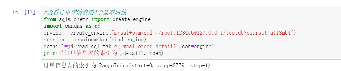

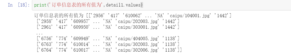
print('All values in the order information table are',detail1.values)

Operation results:

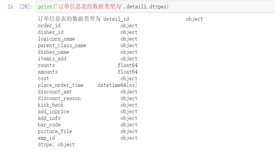
print('The data type of the order information table is',detail1.dtypes)

Operation results:

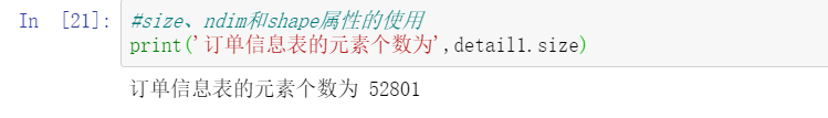
#Use of size, ndim, and shape attributes
print('The number of elements in the order information table is',detail1.size)

Operation results:

print('The dimension number of the order information table is',detail1.ndim)

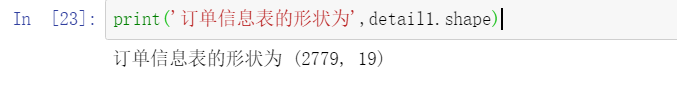
print('The shape of the order information table is',detail1.shape)

Operation results:

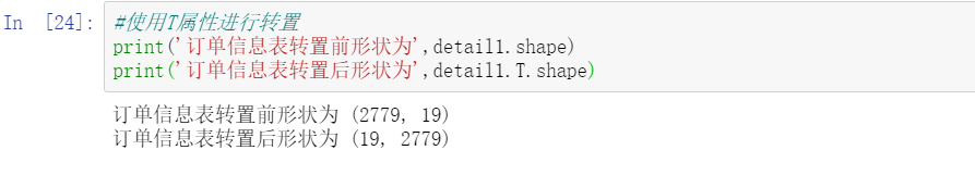
#Transpose using T attribute
print('The shape of the order information table before transposition is',detail1.shape)
print('After the order information table is transposed, the shape is',detail1.T.shape)

Operation results:

4.2.2 finding, adding and deleting DataFrame data

1. View and access data in DataFrame

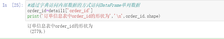
#Access single column data of DataFrame by accessing internal data through dictionary
order_id=detail1['order_id']
print('In the order information table order_id The shape of the is','\n',order_id.shape)

Operation results:

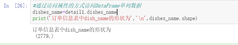
#Access DataFrame single column data by accessing properties
dishes_name=detail1.dishes_name
print('In the order information table dish_name The shape of the is','\n',dishes_name.shape)

Operation results:

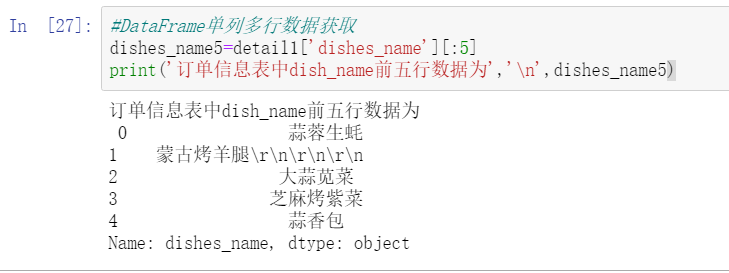
#DataFrame single column and multi row data acquisition
dishes_name5=detail1['dishes_name'][:5]
print('In the order information table dish_name The first five lines of data are','\n',dishes_name5)

Operation results:

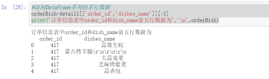
#Accessing multiple rows of data in multiple columns of DataFrame
orderDish=detail1[['order_id','dishes_name']][:5]
print('In the order information table order_id and dish_name The first five lines of data are','\n',orderDish)

Operation results:

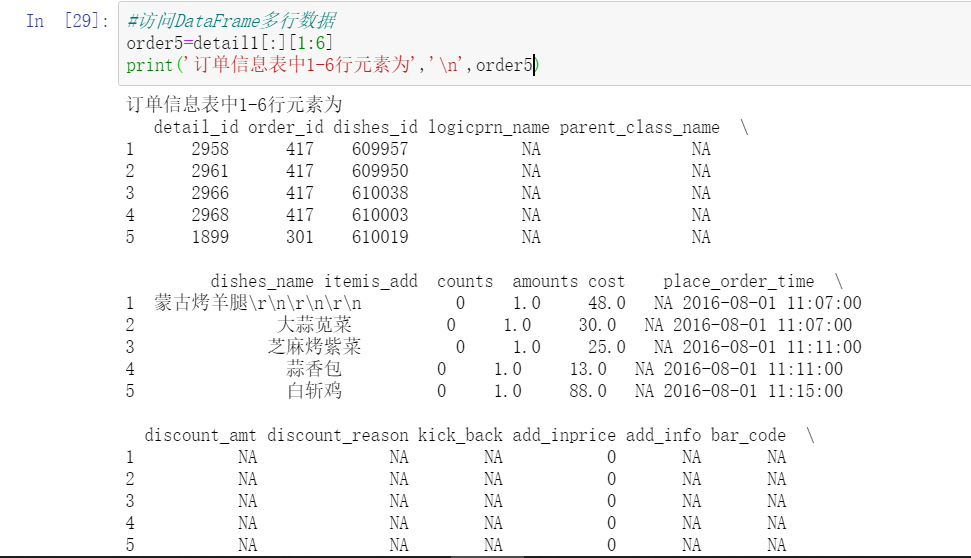
#Accessing multiple rows of DataFrame data
order5=detail1[:][1:6]
print('1 in order information table-6 Row element is','\n',order5)

Operation results:

#Use the head and tail methods of DataFrame to obtain multiple rows of data
print('The first five rows of data in the order information table are','\n',detail1.head())

Operation results:

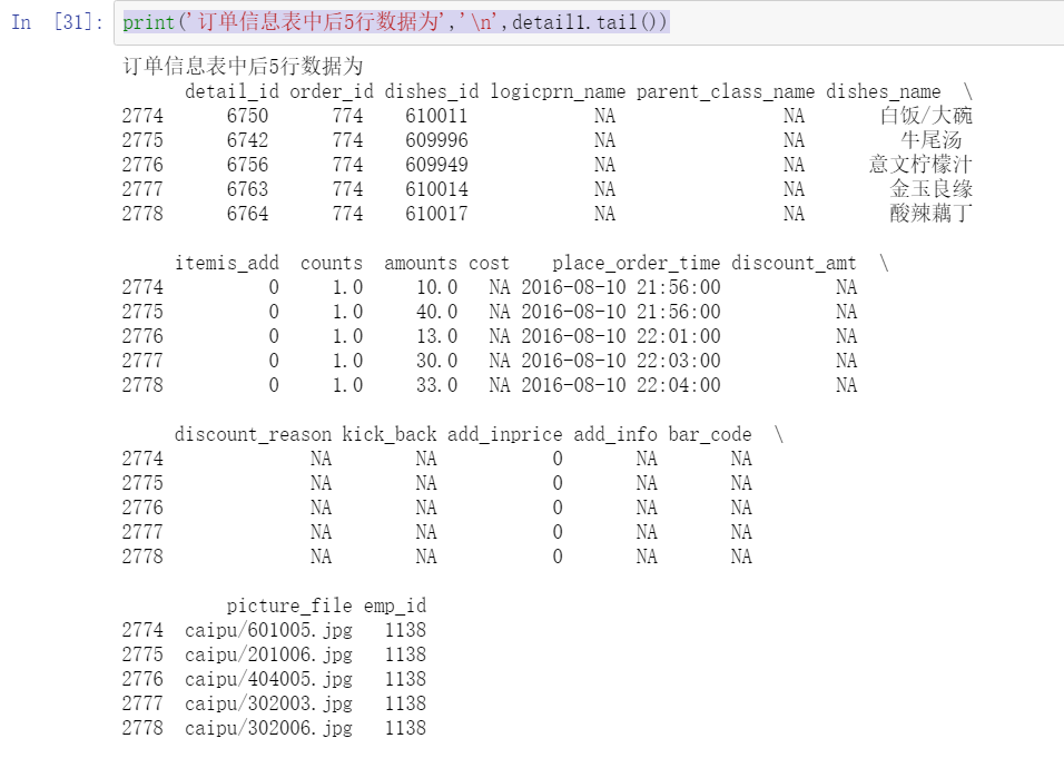
print('The last 5 rows of data in the order information table are','\n',detail1.tail())

Operation results:

#Implementation of single column slicing using loc and iloc
dishes_name1=detail1.loc[:,'dishes_name']
print('use loc extract dishes_name Column size by',dishes_name1.size)
dishes_name2=detail1.iloc[:,3]
print('use loc Extract the of the third column size by',dishes_name2.size)

#Implementation of multi column slicing using loc and iloc
orderDish1=detail1.loc[:,['order_id','dishes_name']]
print('use loc extract order_id and dishes_name Column size by',orderDish1.size)
orderDish2=detail1.iloc[:,[1,3]]
print('use iloc Extract columns 1 and 3 size by',orderDish2.size)

#Using loc and iloc to realize fancy slicing
print('Column name is order_id and dishes_name The data with column name 3 is:\n',detail1.loc[3,['order_id','dishes_name']])
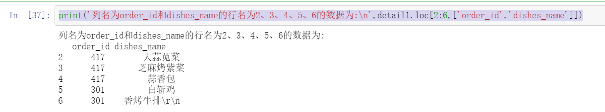
print('Column name is order_id and dishes_name The data with row names 2, 3, 4, 5 and 6 is:\n',detail1.loc[2:6,['order_id','dishes_name']])

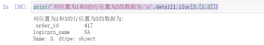
print('The row with column positions 1 and 3 and the data with column position 3 are:\n',detail1.iloc[3,[1,3]])

Operation results:

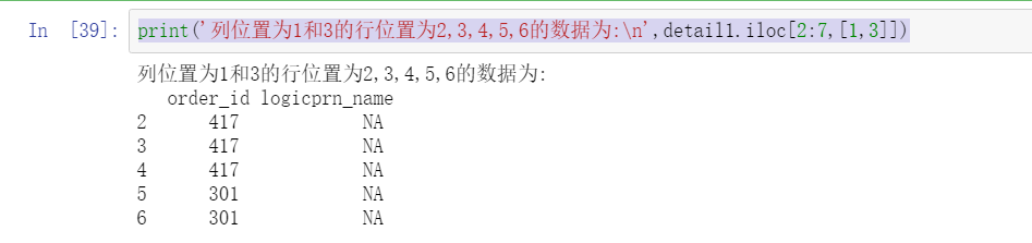
print('The row position with column positions 1 and 3 is 2,3,4,5,6 The data is:\n',detail1.iloc[2:7,[1,3]])

Operation results:

#Implementing conditional slicing using loc and iloc
print('detail in order_id 458 dishes_name by:\n',detail1.loc[detail1['order_id']=='458',['order_id','dishes_name']])

Operation results:

#Using iloc to implement conditional slicing
print('detail in order_id The data in columns 1 and 5 of 458 is:\n',detail1.iloc[(detail1['order_id']=='458').values,[1,5]])

Operation results:

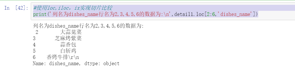
#Using loc,iloc, ix to realize slice comparison
print('Column name is dishes_name The row name is 2,3,4,5,6 The data is:\n',detail1.loc[2:6,'dishes_name'])

Operation results:

print('Column position is 5 and row position is 2-6 The data is:\n',detail1.iloc[2:6,5])

Operation results:

print('Column position is 5 and row position is 2-6 The data is:\n',detail1.ix[2:6,5])

Operation results:

2. Change data in DataFrame

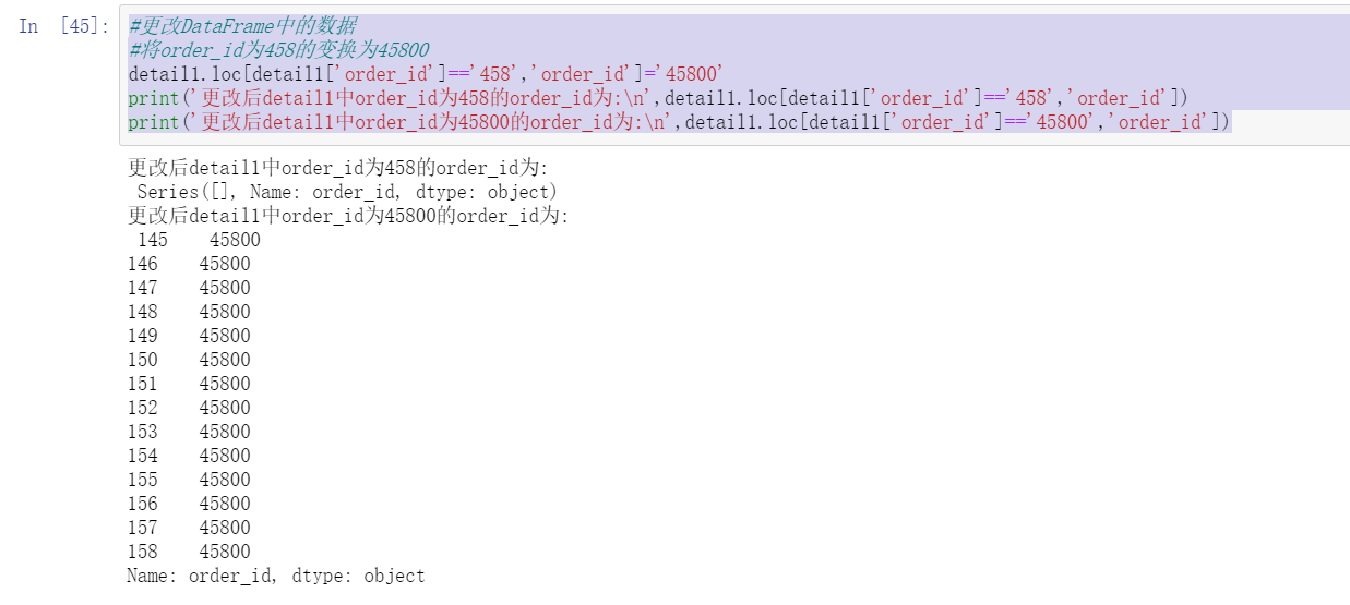
#Change data in DataFrame
#Place order_ The transformation with ID 458 is 45800
detail1.loc[detail1['order_id']=='458','order_id']='45800'
print('After change detail1 in order_id 458 order_id by:\n',detail1.loc[detail1['order_id']=='458','order_id'])
print('After change detail1 in order_id 45800 order_id by:\n',detail1.loc[detail1['order_id']=='45800','order_id'])

Operation results:

3. Add data to DataFrame

#Add a column of non constant values for DataFrame
detail1['payment']=detail1['counts']*detail1['amounts']
print('detail New column payment Top five behaviors of:','\n',detail1['payment'].head())

Operation results:

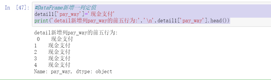
#Add a column of fixed values to DataFrame
detail1['pay_way']='cash payment'
print('detail New column pay_way Top five behaviors of:','\n',detail1['pay_way'].head())

Operation results:

4. Delete a column or row of data

#Delete a DataFrame column
print('delete pay_way front detail The column index of is:','\n',detail1.columns)
detail1.drop(labels='pay_way',axis=1,inplace=True)#label represents the deleted column name, and inplace represents whether it is effective for the original data
print('delete pay_wayde after tail The column index of is:','\n',detail1.columns)

Operation results:

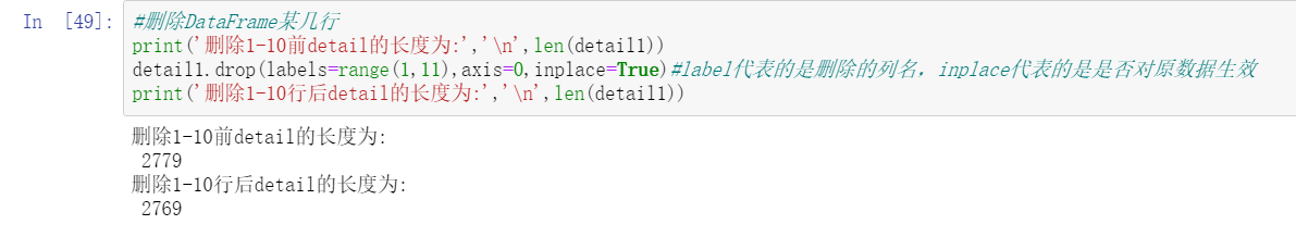
#Delete some rows of DataFrame
print('Delete 1-10 front detail The length of the is:','\n',len(detail1))
detail1.drop(labels=range(1,11),axis=0,inplace=True)#label represents the deleted column name, and inplace represents whether it is effective for the original data
print('Delete 1-10 After line detail The length of the is:','\n',len(detail1))

Operation results:

4.2.3 describe and analyze DataFrame data

1. Descriptive statistics of numerical characteristics

#Use NP The mean function calculates the average price
import numpy as np
print('In the order details table amount(Price)The average value of is',np.mean(detail1['amounts']))

#The covariance matrix calculation of sales volume and price is realized through pandas
print('In the order details table amount(Price)The average value of is',detail1['amounts'].mean())

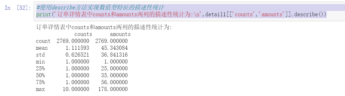
#Use the describe method to realize the descriptive statistics of numerical features
print('In the order details table counts and amounts The descriptive statistics of the two columns are:\n',detail1[['counts','amounts']].describe())

2. Descriptive statistics of category characteristics

#Statistics on the frequency of dish names
print('In the order details table dishes_name The top 10 frequency statistics results are:\n',detail1['dishes_name'].value_counts()[0:10])

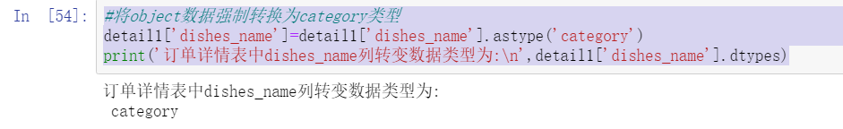
#Cast object data to category type
detail1['dishes_name']=detail1['dishes_name'].astype('category')
print('In the order details table dishes_name Column transition data type is:\n',detail1['dishes_name'].dtypes)

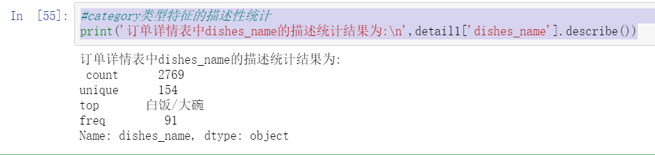
#Descriptive statistics of category type characteristics
print('In the order details table dishes_name The descriptive statistical results are:\n',detail1['dishes_name'].describe())

4.2.4 task realization

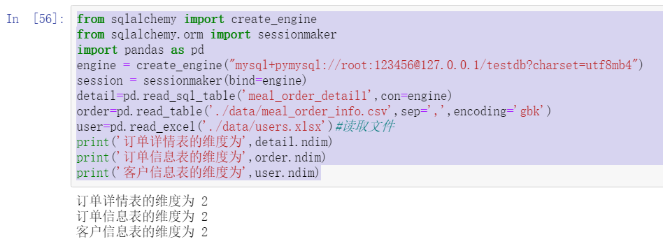
1. View the size and dimension of catering data

from sqlalchemy import create_engine
from sqlalchemy.orm import sessionmaker
import pandas as pd
engine = create_engine("mysql+pymysql://root:123456@127.0.0.1/testdb?charset=utf8mb4")
session = sessionmaker(bind=engine)
detail=pd.read_sql_table('meal_order_detail1',con=engine)
order=pd.read_table('./data/meal_order_info.csv',sep=',',encoding='gbk')
user=pd.read_excel('./data/users.xlsx')#read file
print('The dimension of the order details table is',detail.ndim)
print('The dimension of the order information table is',order.ndim)
print('The dimension of the customer information table is',user.ndim)

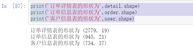
print('The shape of the order details table is',detail.shape)
print('The shape of the order information table is',order.shape)
print('The shape of the customer information table is',user.shape)

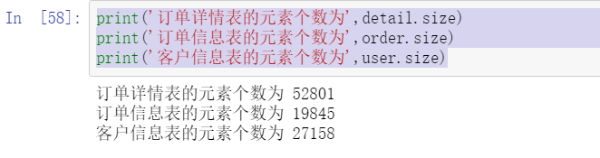
print('The number of elements in the order details table is',detail.size)
print('The number of elements in the order information table is',order.size)
print('The number of elements in the customer information table is',user.size)

2. Statistics of catering dish sales

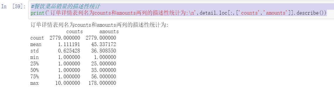
#Descriptive statistics of catering dish sales
print('The order details table is listed as counts and amounts The descriptive statistics of the two columns are:\n',detail.loc[:,['counts','amounts']].describe())

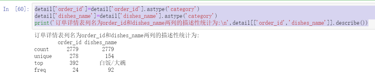
detail['order_id']=detail['order_id'].astype('category')
detail['dishes_name']=detail['dishes_name'].astype('category')
print('The order details table is listed as order_id and dishes_name The descriptive statistics of the two columns are:\n',detail[['order_id','dishes_name']].describe())

3. Columns with all null values or the same values of all elements are excluded

#Exclude the entire column of catering dishes that is empty or has the same value
#Define a function to eliminate columns with null values and columns with standard deviation of 0
def dropNullStd(data):
    beforelen=data.shape[1]
    colisNull=data.describe().loc['count']==0
    for i in range(len(colisNull)):
        if colisNull[i]:
            data.drop(colisNull.index[i],axis=1,inplace=True)
    stdisZero=data.describe().loc['std']==0
    for i in range(len(stdisZero)):
        if stdisZero[i]:
            data.drop(stdisZero.index[i],axis=1,inplace=True)
    afterlen=data.shape[1]
    print('The number of columns culled is:', beforelen-afterlen)
    print('The shape of the data after elimination is:',data.shape)
dropNullStd(detail)

#Use the dropNullStd function to operate on the order information table
dropNullStd(order)

#Use the dropNullStd function to operate on the customer information table
dropNullStd(user)

Task 4.3 converting and processing time series data

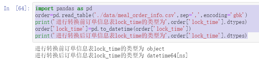
4.3.1 convert string time to standard time

Timestamp is the most basic and commonly used time class. In most cases, it will convert time related strings into timestamp. pandas provides to_datetime function implementation

import pandas as pd
order=pd.read_table('./data/meal_order_info.csv',sep=',',encoding='gbk')
print('Order information table before conversion lock_time The type of is',order['lock_time'].dtypes)
order['lock_time']=pd.to_datetime(order['lock_time'])
print('Order information table after conversion lock_time The type of is',order['lock_time'].dtypes)

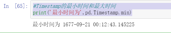
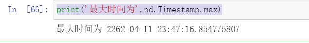
The time of Timestamp type is limited. It can only be expressed to September 21, 1677 at the earliest and April 11, 2262 at the latest

#Minimum and maximum time of Timestamp
print('The minimum time is',pd.Timestamp.min)

print('The maximum time is',pd.Timestamp.max)

#The time string is converted to DatatimeIndex and PeriodIndex
dateIndex=pd.DatetimeIndex(order['lock_time'])

print('Order information table after conversion lock_time The type of is',type(dateIndex))

print(order["lock_time"])
periods = pd.PeriodIndex(lock_time=order["lock_time"],freq="H")
print('Order information table after conversion lock_time The type of is',type(periods))

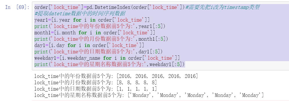
4.3.2 extracting time series data information

order['lock_time']=pd.DatetimeIndex(order['lock_time'])#You need to change i to timestamp type first
#Extract time series data from datetime data
year1=[i.year for i in order['lock_time']]
print('lock_time The first 5 years in the data are:',year1[:5])
month1=[i.month for i in order['lock_time']]
print('lock_time The first 5 months of data in are:',month1[:5])
day1=[i.day for i in order['lock_time']]
print('lock_time The first 5 dates in are:',day1[:5])
weekday1=[i.weekday_name for i in order['lock_time']]
print('lock_time The first 5 days of the week name data in are:',weekday1[:5])

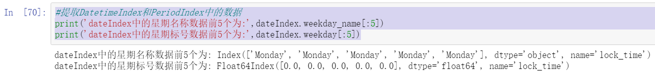
#Extract data from DatetimeIndex and PeriodIndex
print('dateIndex The first 5 days of the week name data in are:',dateIndex.weekday_name[:5])
print('dateIndex The first 5 days of week label data in are:',dateIndex.weekday[:5])

4.3.3 addition and subtraction time data

#Using Timedelta to realize the addition of time data
#lock_time data is shifted back one day
time1=order['lock_time']+pd.Timedelta(days=1)
print('lock_time Add the first five rows of data a day ago:\n',order['lock_time'][:5])
print('lock_time Add the first five rows of data a day ago:\n',time1[:5])

#Using Timedelta to realize the subtraction operation of time data
timeDelta=order['lock_time']-pd.to_datetime('2017-1-1')
print('lock_time Minus the data after 0:00:00 on January 1, 2017:\n',timeDelta[:5])
print('lock_time subtract time1 The data type after is:\n',timeDelta.dtypes)

#Time data conversion of order information table
import pandas as pd
order=pd.read_table('./data/meal_order_info.csv',sep=',',encoding='gbk')
print('Order information table before conversion user_start_time and lock_time The type of is:\n',order[['use_start_time','lock_time']].dtypes)
order['use_start_time']=pd.to_datetime(order['use_start_time'])
order['lock_time']=pd.to_datetime(order['lock_time'])
print('Order information table after conversion user_start_time and lock_time The type of is:\n',order[['use_start_time','lock_time']].dtypes)

2. Extract the month, day and week information in the dish data

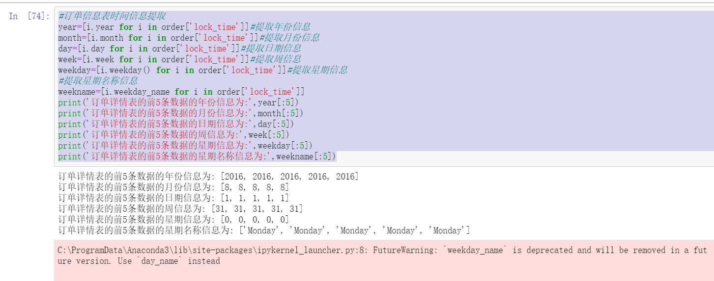
#Order information table time information extraction
year=[i.year for i in order['lock_time']]#Extract year information
month=[i.month for i in order['lock_time']]#Extract month information
day=[i.day for i in order['lock_time']]#Extract date information
week=[i.week for i in order['lock_time']]#Extract weekly information
weekday=[i.weekday() for i in order['lock_time']]#Extract week information
#Extract week name information
weekname=[i.weekday_name for i in order['lock_time']]
print('The year information of the first five data in the order details table is:',year[:5])
print('The month information of the first five data in the order details table is:',month[:5])
print('The date information of the first five items of data in the order details table is:',day[:5])
print('The weekly information of the first five data in the order details table is:',week[:5])
print('The week information of the first five data in the order details table is:',weekday[:5])
print('The week name information of the first five data in the order details table is:',weekname[:5])

3. View time statistics in order information table

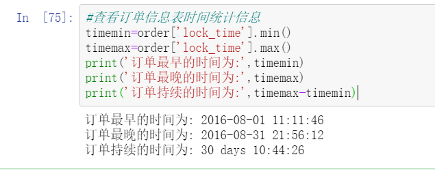
#View time statistics in order information table
timemin=order['lock_time'].min()
timemax=order['lock_time'].max()
print('The earliest time of order is:',timemin)
print('The latest time of order is:',timemax)
print('The order duration is:',timemax-timemin)

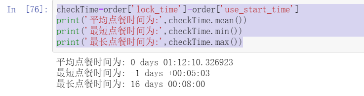
checkTime=order['lock_time']-order['use_start_time']
print('The average ordering time is:',checkTime.mean())
print('The shortest ordering time is:',checkTime.min())
print('The maximum order time is:',checkTime.max())

Task 4.4 intra group calculation using group aggregation

4.4.1 splitting data using group by method

#The order details of dishes are grouped according to the order number
import pandas as pd
import numpy as np
from sqlalchemy import create_engine
from sqlalchemy.orm import sessionmaker

engine = create_engine("mysql+pymysql://root:123456@127.0.0.1/testdb?charset=utf8mb4")
session = sessionmaker(bind=engine)
detail=pd.read_sql_table('meal_order_detail1',con=engine)
detailGroup=detail[['order_id','counts','amounts']].groupby(by='order_id')
print('The order detail table after grouping is',detailGroup)
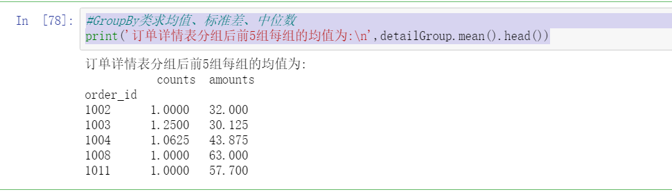
#GroupBy class calculates the mean, standard deviation and median
print('After the order details table is grouped, the average value of each group of the first five groups is:\n',detailGroup.mean().head())
print('The standard deviation of each group of the first five groups after grouping the order details table is:\n',detailGroup.std().head())
print('After the order details table is grouped, the size of the first 5 groups is:\n',detailGroup.size().head())

4.4.2 aggregating data using agg method

#Use agg to find the statistics corresponding to the current data
print('The sum and average of the sales volume and selling price of dishes in the order details table is:\n',detail[['counts','amounts']].agg([np.sum,np.mean]))

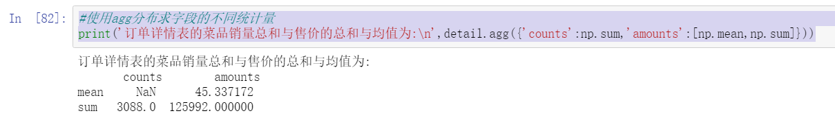
#Using agg distribution to find different statistics of fields
print('The sum and average of the total sales volume and selling price of dishes in the order details table are:\n',detail.agg({'counts':np.sum,'amounts':[np.mean,np.sum]}))

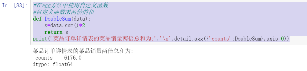
#Using custom functions in agg methods
#Double the sum of custom functions
def DoubleSum(data):
    s=data.sum()*2
    return s
print('The sum of twice the sales volume of dishes in the dish order details table is:','\n',detail.agg({'counts':DoubleSum},axis=0))

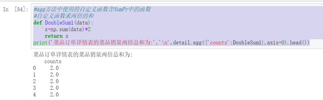
#The custom functions used in the agg method include those in NumPy
#Double the sum of custom functions
def DoubleSum1(data):
    s=np.sum(data)*2
    return s
print('The sum of twice the sales volume of dishes in the dish order details table is:','\n',detail.agg({'counts':DoubleSum1},axis=0).head())

print('After the order details table is grouped, the average value of each group of the first three groups is:\n',detailGroup.agg(np.mean).head(3))

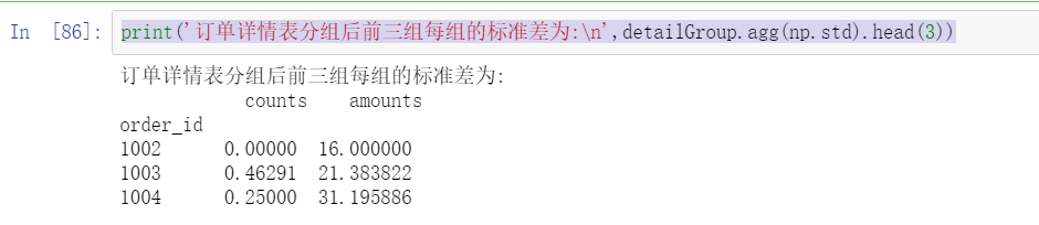
print('After the order details table is grouped, the standard deviation of the first three groups is:\n',detailGroup.agg(np.std).head(3))

#Use agg method to use different aggregation functions for grouped data
print('After the order details table is grouped, the average value of the total number of dishes and selling price of each group in the first three groups is:\n',detailGroup.agg({'counts':np.sum,'amounts':np.mean}).head(3))

4.4.3 aggregate data using the apply method

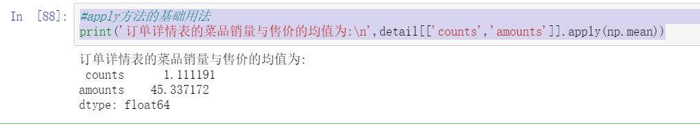
#Basic usage of apply method
print('The average sales volume and selling price of dishes in the order details table are:\n',detail[['counts','amounts']].apply(np.mean))

#Aggregate using the apply method
print('The average value of the first three groups in the order details table is:\n',detailGroup.apply(np.mean).head(3))

print('Standard deviation of the first three groups of order details:\n',detailGroup.apply(np.std).head(3))

4.4.4 aggregate data using transform method

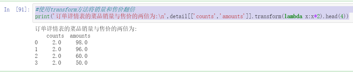
#Use the transform method to double the sales volume and selling price
print('The sales volume of dishes in the order details table is twice the selling price:\n',detail[['counts','amounts']].transform(lambda x:x*2).head(4))

#Standardization of intra group dispersion using transform
print('After grouping the order detail table, the first 5 behaviors after realizing the dispersion standardization within the group:\n',detailGroup.transform(lambda x:(x.mean()-x.min())/(x.max()-x.min())).head())

4.4.5 task realization

1. Split the dish order details table according to the time

#The order details table is grouped by date
import pandas as pd
import numpy as np
from sqlalchemy import create_engine
from sqlalchemy.orm import sessionmaker

engine = create_engine("mysql+pymysql://root:123456@127.0.0.1/testdb?charset=utf8mb4")
session = sessionmaker(bind=engine)
detail=pd.read_sql_table('meal_order_detail1',con=engine)
detail['place_order_time']=pd.to_datetime(detail['place_order_time'])
detail['date']=[i.date() for i in detail['place_order_time']]
detailGroup=detail[['date','counts','amounts']].groupby(by='date')
print('The number of the first 5 groups in the order details table is:\n',detailGroup.size().head())

2. The average unit price and median selling price of dishes sold in a single day were calculated by agg method

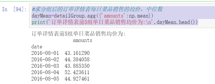
#Find the average price and median of daily dish sales in the order details table after grouping
dayMean=detailGroup.agg({'amounts':np.mean})
print('The average selling price of the first five groups of single day dishes in the order details table is:\n',dayMean.head())

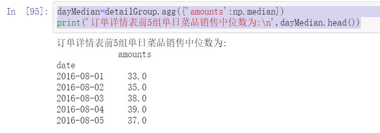
dayMedian=detailGroup.agg({'amounts':np.median})
print('The median sales of the first five groups of single day dishes in the order details table is:\n',dayMedian.head())

3. Use the apply method to count the number of dishes sold in a single day

#Get the total sales volume of daily dishes in the order details table
daySaleSum=detailGroup.apply(np.sum)['counts']
print('The number of dishes sold in the first five groups of one-day dishes in the order details table is:\n',daySaleSum.head())

Task 4.5 create PivotTable and crosstab

4.5.11 using pivot_ Create pivot table with table function

#Use the order number as the pivot table index to make a pivot chart
import pandas as pd
import numpy as np
from sqlalchemy import create_engine
from sqlalchemy.orm import sessionmaker

engine = create_engine("mysql+pymysql://root:123456@127.0.0.1/testdb?charset=utf8mb4")
session = sessionmaker(bind=engine)
detail=pd.read_sql_table('meal_order_detail1',con=engine)
detailPivot=pd.pivot_table(detail[['order_id','counts','amounts']],index='order_id')
print('with order_id Order PivotTable created as a grouping key:\n',detailPivot.head())

#Pivot table after modifying aggregate function
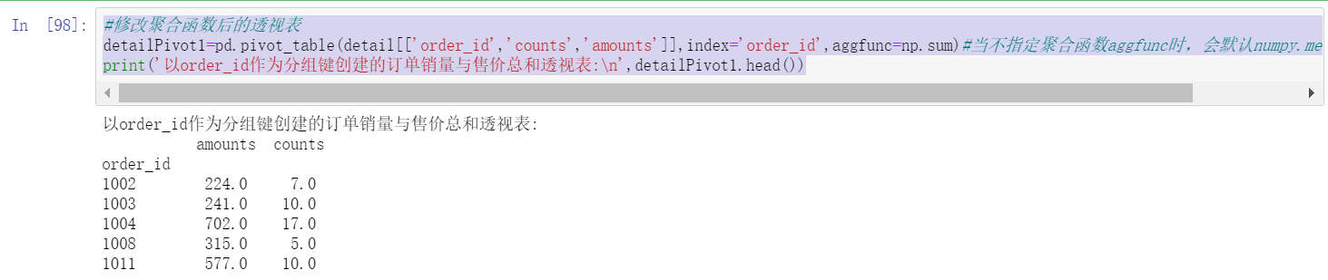
detailPivot1=pd.pivot_table(detail[['order_id','counts','amounts']],index='order_id',aggfunc=np.sum)#When the aggregate function aggfunc is not specified, numpy. Is defaulted Aggregate calculation by mean
print('with order_id Pivot table of the sum of order sales volume and selling price created as a grouping key:\n',detailPivot1.head())

#Pivot table with order number and dish name as index
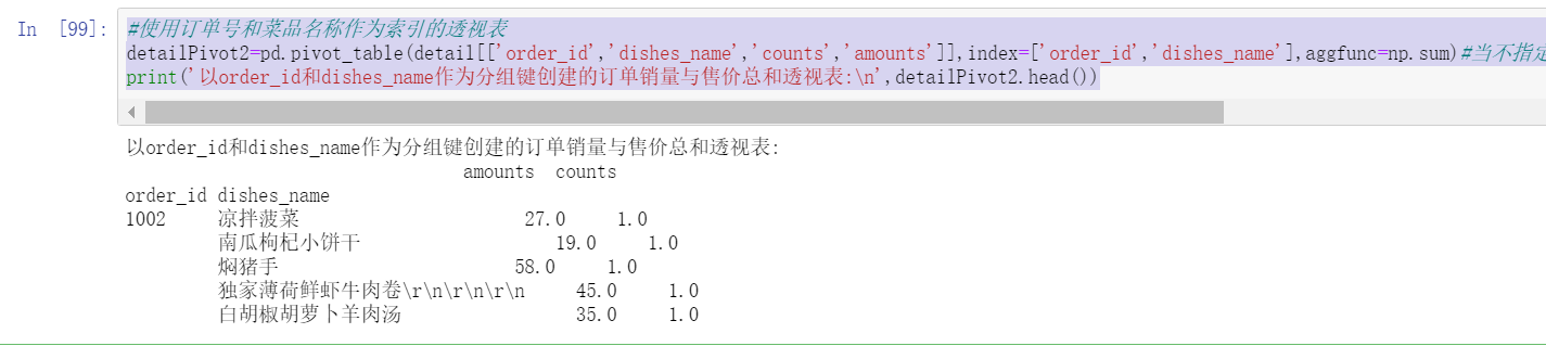
detailPivot2=pd.pivot_table(detail[['order_id','dishes_name','counts','amounts']],index=['order_id','dishes_name'],aggfunc=np.sum)#When the aggregate function aggfunc is not specified, numpy. Is defaulted Aggregate calculation by mean
print('with order_id and dishes_name Pivot table of the sum of order sales volume and selling price created as a grouping key:\n',detailPivot2.head())

#Pivot table with specified dish name as column grouping key
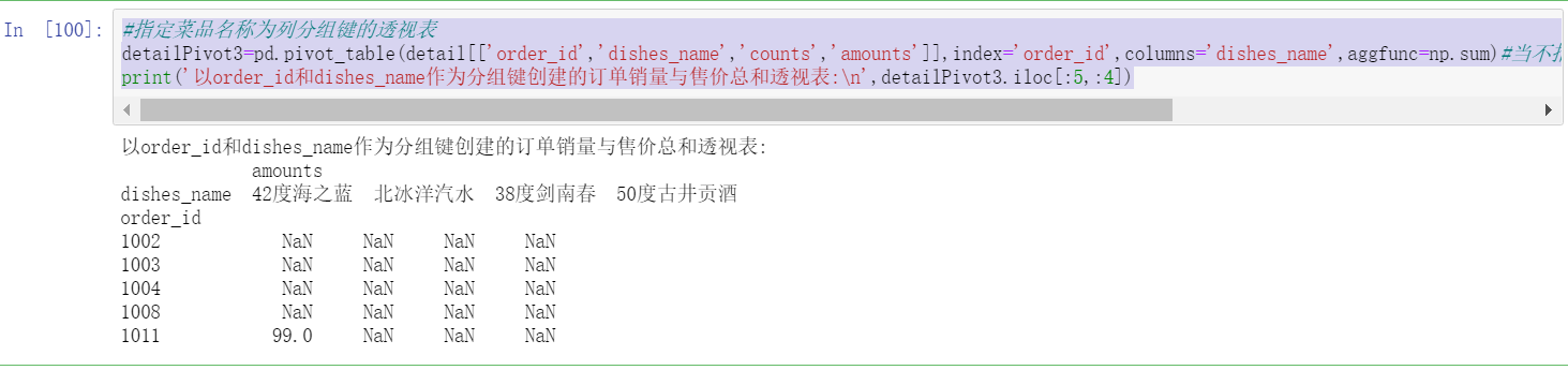
detailPivot3=pd.pivot_table(detail[['order_id','dishes_name','counts','amounts']],index='order_id',columns='dishes_name',aggfunc=np.sum)#When the aggregate function aggfunc is not specified, numpy. Is defaulted Aggregate calculation by mean
print('with order_id and dishes_name Pivot table of the sum of order sales volume and selling price created as a grouping key:\n',detailPivot3.iloc[:5,:4])

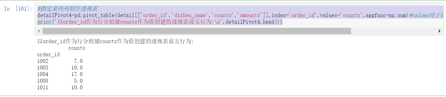
#Specify some columns to make a PivotTable report
detailPivot4=pd.pivot_table(detail[['order_id','dishes_name','counts','amounts']],index='order_id',values='counts',aggfunc=np.sum)#values is used to specify the name of the data field to be aggregated. All data is used by default
print('with order_id As row grouping key counts Top five pivot table behaviors created as values:\n',detailPivot4.head())

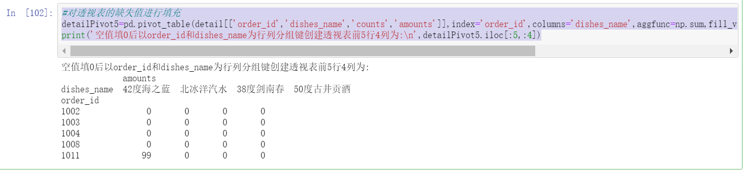
#Fill in the missing values of the pivot table
detailPivot5=pd.pivot_table(detail[['order_id','dishes_name','counts','amounts']],index='order_id',columns='dishes_name',aggfunc=np.sum,fill_value=0)#values is used to specify the name of the data field to be aggregated. All data is used by default
print('Fill in the blank value with 0 and then order_id and dishes_name The first 5 rows and 4 columns of the pivot table created for row column grouping keys are:\n',detailPivot5.iloc[:5,:4])

#Add to PivotTable summary
detailPivot6=pd.pivot_table(detail[['order_id','dishes_name','counts','amounts']],index='order_id',columns='dishes_name',aggfunc=np.sum,fill_value=0,margins=True)
#margins indicates the switch of the summary function. When set to True, rows and columns named ALL will appear in the result set. The default is True
print('Fill in the blank value with 0 and then order_id and dishes_name The first 5 rows and 4 columns of the pivot table created for row column grouping keys are:\n',detailPivot6.iloc[:5,-4:])

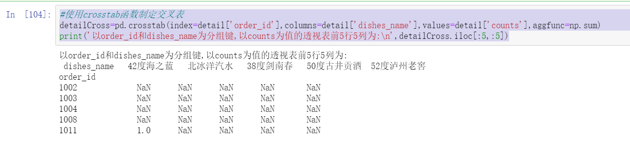
4.5.2 create a crosstab using the crosstab function

#Use the crosstab function to make a cross table
detailCross=pd.crosstab(index=detail['order_id'],columns=detail['dishes_name'],values=detail['counts'],aggfunc=np.sum)
print('with order_id and dishes_name Group key,with counts The first 5 rows and 5 columns of the PivotTable with values are:\n',detailCross.iloc[:5,:5])

4.5.3 task realization

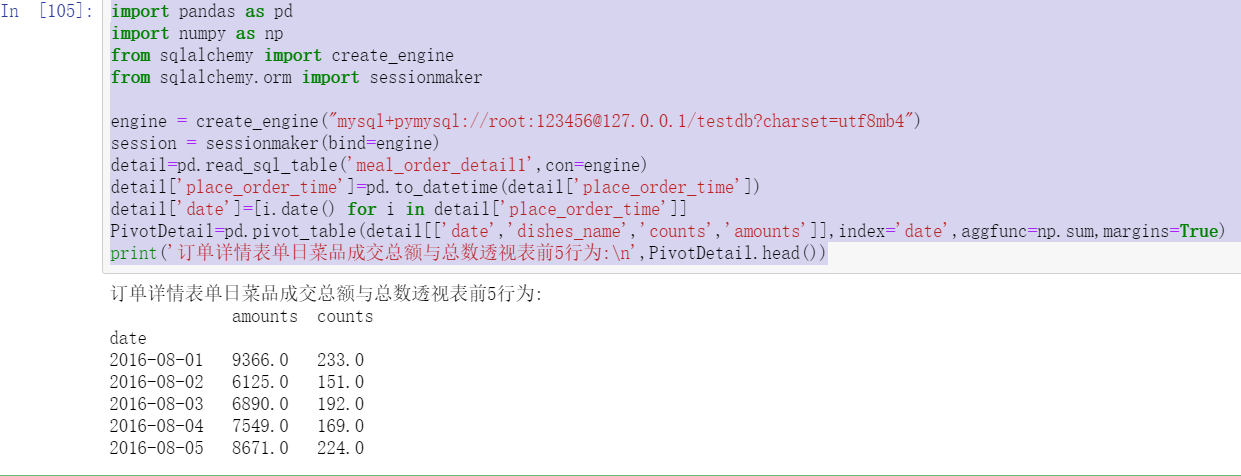
1. Create a daily menu transaction total and average price PivotTable

import pandas as pd
import numpy as np
from sqlalchemy import create_engine
from sqlalchemy.orm import sessionmaker

engine = create_engine("mysql+pymysql://root:123456@127.0.0.1/testdb?charset=utf8mb4")
session = sessionmaker(bind=engine)
detail=pd.read_sql_table('meal_order_detail1',con=engine)
detail['place_order_time']=pd.to_datetime(detail['place_order_time'])
detail['date']=[i.date() for i in detail['place_order_time']]
PivotDetail=pd.pivot_table(detail[['date','dishes_name','counts','amounts']],index='date',aggfunc=np.sum,margins=True)
print('Top 5 behaviors of daily dish transaction amount and total amount pivot table in order details form:\n',PivotDetail.head())

2. Create a pivot table of the total transaction amount of a single dish in a single day

#Order details form pivot table of daily transaction amount of each dish
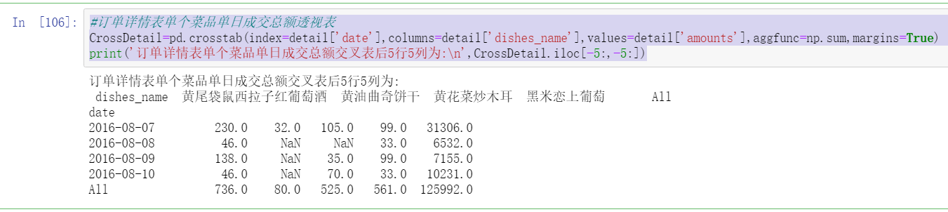
CrossDetail=pd.crosstab(index=detail['date'],columns=detail['dishes_name'],values=detail['amounts'],aggfunc=np.sum,margins=True)
print('5 rows and 5 columns after the cross table of daily transaction amount of each dish in the order details form:\n',CrossDetail.iloc[-5:,-5:])

Practical training

Training 1 read and view the basic information of P2P network loan data master table

1. View the size, dimension and memory of the data

import pandas as pd
import numpy as np
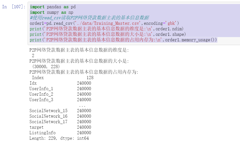
#Using read_csv reads the basic information data of the P2P network loan data master table
order1=pd.read_csv('./data/Training_Master.csv',encoding='gbk')
print('P2P The dimension of basic information data in the main table of online loan data is:\n',order1.ndim)
print('P2P The size of the basic information data in the main table of network loan data is:\n',order1.shape)
print('P2P The memory occupied by the basic information data of the main table of network loan data is:\n',order1.memory_usage())

2. Descriptive statistics of data

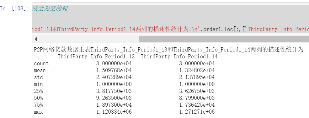
#Use the describe method for descriptive statistics, and eliminate the columns with the same value or all empty values
# print(order1.columns)
#User third-party platform information
print('P2P Main table of online loan data ThirdParty_Info_Period1_13 and ThirdParty_Info_Period1_14 The descriptive statistics of the two columns are:\n',order1.loc[:,['ThirdParty_Info_Period1_13','ThirdParty_Info_Period1_14']].describe())

order1['Idx']=order1['Idx'].astype('category')#User ID
order1['UserInfo_2']=order1['UserInfo_2'].astype('category')#Basic user information
print('''P2P Main table of online loan data Idx And UserInfo_2 The descriptive statistical results are:''','\n',order1[['Idx','UserInfo_2']].describe())

3. Columns with all null values or the same values of all elements are excluded

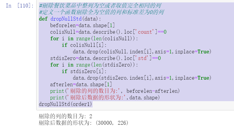
#Exclude the entire column of catering dishes that is empty or has the same value
#Define a function to eliminate columns with null values and columns with standard deviation of 0
def dropNullStd(data):
    beforelen=data.shape[1]
    colisNull=data.describe().loc['count']==0
    for i in range(len(colisNull)):
        if colisNull[i]:
            data.drop(colisNull.index[i],axis=1,inplace=True)
    stdisZero=data.describe().loc['std']==0
    for i in range(len(stdisZero)):
        if stdisZero[i]:
            data.drop(stdisZero.index[i],axis=1,inplace=True)
    afterlen=data.shape[1]
    print('The number of columns culled is:', beforelen-afterlen)
    print('The shape of the data after elimination is:',data.shape)
dropNullStd(order1)

Training 2 extract the time information of user information update table and login information table

1. Convert string time to standard time

import pandas as pd
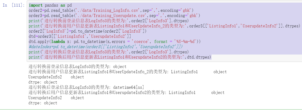
order2=pd.read_table('./data/Training_LogInfo.csv',sep=',',encoding='gbk')
order3=pd.read_table('./data/Training_Userupdate.csv',sep=',',encoding='gbk')
print('Login information table before conversion LogInfo3 The type of is:',order2['LogInfo3'].dtypes)
print('User information update table before conversion ListingInfo1 and UserUpdateInfo_2 The type of is:',order3[['ListingInfo1','UserupdateInfo2']].dtypes)
order2['LogInfo3']=pd.to_datetime(order2['LogInfo3'])
dtd=order3[['ListingInfo1','UserupdateInfo2']]
dtd.apply(lambda x: pd.to_datetime(x,errors = 'coerce', format = '%Y-%m-%d'))
#dateIndex=pd.to_datetime(order3[['ListingInfo1','UserupdateInfo2']])
print('Login information table after conversion LogInfo3 The type of is:',order2['LogInfo3'].dtypes)
print('User information update table after conversion ListingInfo1 and UserupdateInfo2 The type of is:',dtd.dtypes)

2. Use year, month, week and other methods to extract the time information in the user information table and login information table

#Extract the time information of the login information table
year1=[i.year for i in order2['LogInfo3']]
print('LogInfo3 The first 5 years in the data are:',year1[:5])
month1=[i.month for i in order2['LogInfo3']]
print('LogInfo3 The first 5 months of data in are:',month1[:5])
day1=[i.day for i in order2['LogInfo3']]
print('LogInfo3 The first 5 dates in are:',day1[:5])
weekday1=[i.weekday_name for i in order2['LogInfo3']]
print('LogInfo3 The first 5 days of the week name data in are:',weekday1[:5])

#Extract the time information of the user information table
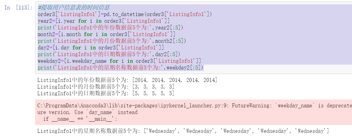
order3['ListingInfo1']=pd.to_datetime(order3['ListingInfo1'])
year2=[i.year for i in order3['ListingInfo1']]
print('ListingInfo1 The first 5 years in the data are:',year2[:5])
month2=[i.month for i in order3['ListingInfo1']]
print('ListingInfo1 The first 5 months of data in are:',month2[:5])
day2=[i.day for i in order3['ListingInfo1']]
print('ListingInfo1 The first 5 dates in are:',day2[:5])
weekday2=[i.weekday_name for i in order3['ListingInfo1']]
print('ListingInfo1 The first 5 days of the week name data in are:',weekday2[:5])

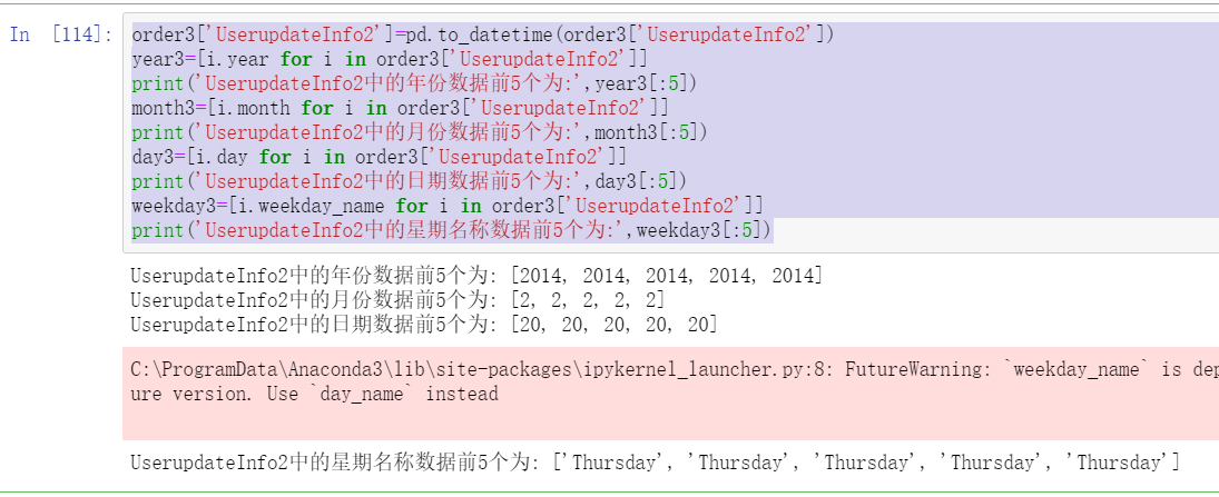
order3['UserupdateInfo2']=pd.to_datetime(order3['UserupdateInfo2'])
year3=[i.year for i in order3['UserupdateInfo2']]
print('UserupdateInfo2 The first 5 years in the data are:',year3[:5])
month3=[i.month for i in order3['UserupdateInfo2']]
print('UserupdateInfo2 The first 5 months of data in are:',month3[:5])
day3=[i.day for i in order3['UserupdateInfo2']]
print('UserupdateInfo2 The first 5 dates in are:',day3[:5])
weekday3=[i.weekday_name for i in order3['UserupdateInfo2']]
print('UserupdateInfo2 The first 5 days of the week name data in are:',weekday3[:5])

3. Calculate the time difference between the user information table and the login information table in days, hours and minutes respectively

import numpy as np
# year1=np.array(year1)
# print(year1)
# year2=np.array(year2)
# print(year2)
# time_year=year1-year2
dayDelta=order3['ListingInfo1']-order2['LogInfo3']#In days
print("The calculation time difference is in days:\n",dayDelta.head())
def TransformhourDelta(data):
    for i in range(0,len(data)):
        data[i]=data[i].total_seconds()/3600
    return data
print("The calculation time difference is in hours:\n",TransformhourDelta(dayDelta).head())
def TransformDayIntoMinute(data):
    for i in range(0,len(data)):
        data[i]=data[i].total_seconds()/60
    return data 
timeDeltaUserupdate=order3["ListingInfo1"]-order2['LogInfo3']
print("The calculation time difference is in minutes:\n",TransformDayIntoMinute(timeDeltaUserupdate).head())

Training 3 uses grouping aggregation method to further analyze user information update table and login information table

1. Splitting data using the group by method

import pandas as pd
import numpy as np
from sqlalchemy import create_engine
from sqlalchemy.orm import sessionmaker

engine = create_engine("mysql+pymysql://root:123456@127.0.0.1/testdb?charset=utf8mb4")
session = sessionmaker(bind=engine)
order2=pd.read_table('./data/Training_LogInfo.csv',sep=',',encoding='gbk')
order3=pd.read_table('./data/Training_Userupdate.csv',sep=',',encoding='gbk')
order2Group=order2[['Idx','Listinginfo1','LogInfo1','LogInfo2','LogInfo3']].groupby(by='Idx')
print('The login information table after grouping is',order2Group)

order3Group=order3[['Idx','ListingInfo1','UserupdateInfo1','UserupdateInfo2']].groupby(by='Idx')
print('The user information update table after grouping is',order3Group)
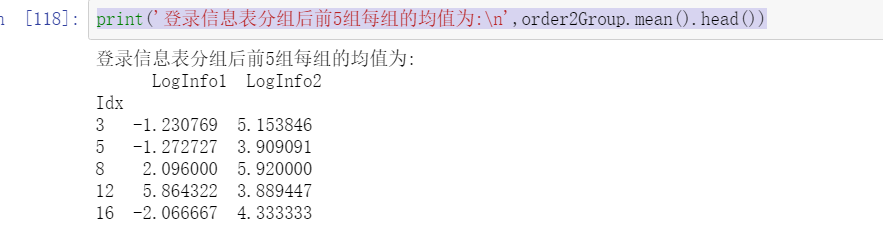
print('After the login information table is grouped, the average value of each group of the first five groups is:\n',order2Group.mean().head())

print('After the login information table is grouped, the standard deviation of each group of the first five groups is:\n',order2Group.std().head())

print('After the login information table is grouped, the size of the first five groups is:\n',order2Group.size().head())

print('After grouping the user information update table, the average value of each group of the first five groups is:\n',order3Group.mean().head())

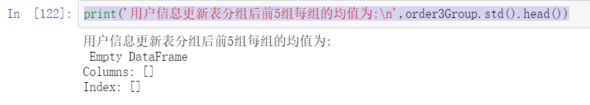
print('After grouping the user information update table, the average value of each group of the first five groups is:\n',order3Group.std().head())

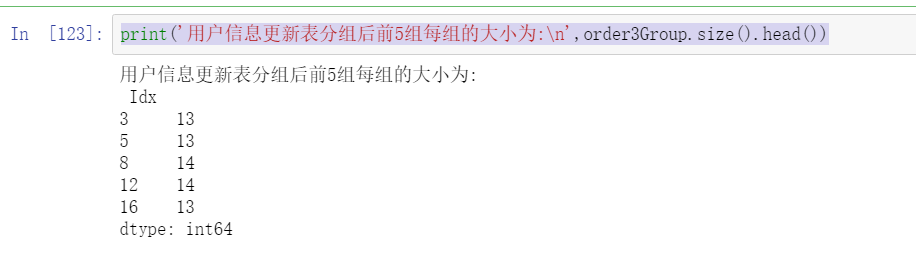
print('After grouping the user information update table, the size of each of the first five groups is:\n',order3Group.size().head())

2. Use agg method to calculate the earliest and latest update and login time after grouping

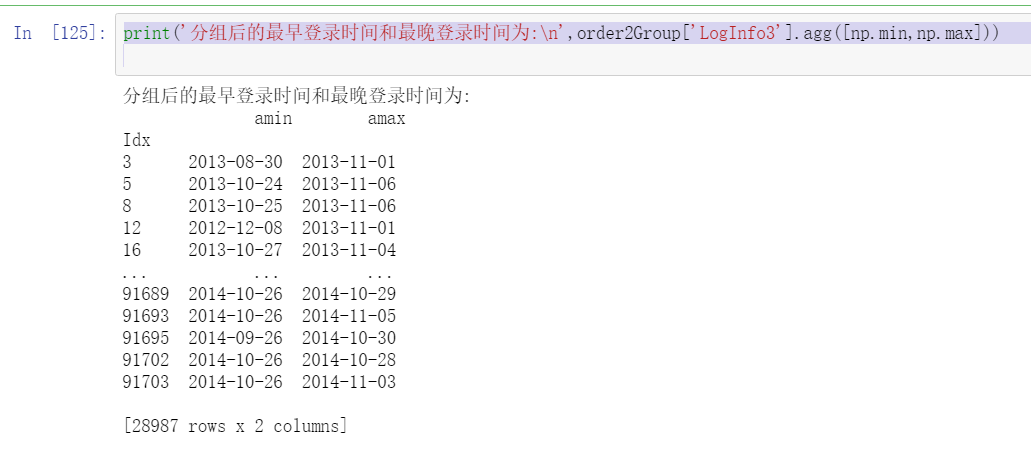
print('The earliest login time and the latest login time after grouping are:\n',order2Group['LogInfo3'].agg([np.min,np.max]))

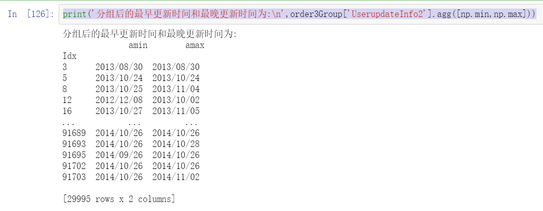
print('The earliest update time and the latest update time after grouping are:\n',order3Group['UserupdateInfo2'].agg([np.min,np.max]))

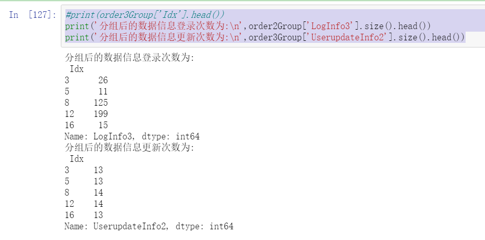
3. Use the size method to calculate the information update times and login times of the grouped data

#print(order3Group['Idx'].head())
print('The login times of data information after grouping are:\n',order2Group['LogInfo3'].size().head())
print('The number of data information updates after grouping is:\n',order3Group['UserupdateInfo2'].size().head())

Training 4: convert the length width table of user information update table and login information table

1. Using pivot_table function to convert length width table

import pandas as pd
import numpy as np
from sqlalchemy import create_engine
from sqlalchemy.orm import sessionmaker

engine = create_engine("mysql+pymysql://root:123456@127.0.0.1/testdb?charset=utf8mb4")
session = sessionmaker(bind=engine)
order2=pd.read_table('./data/Training_LogInfo.csv',sep=',',encoding='gbk')
order3=pd.read_table('./data/Training_Userupdate.csv',sep=',',encoding='gbk')
order2Pivot=pd.pivot_table(order2[['Idx','Listinginfo1','LogInfo1','LogInfo2','LogInfo3']],index='Idx',aggfunc=np.sum)
print('with Idx The login information table created for the sub key group is:\n',order2Pivot.head())
order3Pivot=pd.pivot_table(order3[['Idx','ListingInfo1','UserupdateInfo1','UserupdateInfo2']],index='Idx',aggfunc=np.sum)
print('with Idx The information update table created for the sub key group is:\n',order3Pivot.head())

#Pivot table indexed by user identifier and login time
order2Pivot=pd.pivot_table(order2[['Idx','Listinginfo1','LogInfo1','LogInfo2','LogInfo3']],index=['Idx','Listinginfo1'],aggfunc=np.sum)
print('with Idx and Listinginfo1 The login information table created for the sub key group is:\n',order2Pivot.head())
order3Pivot=pd.pivot_table(order3[['Idx','ListingInfo1','UserupdateInfo1','UserupdateInfo2']],index=['Idx','ListingInfo1'],aggfunc=np.sum)
print('with Idx and ListingInfo1 The information update table created for the sub key group is:\n',order3Pivot.head())

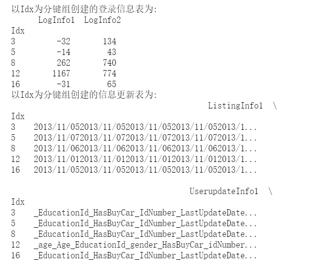
order2Pivot=pd.pivot_table(order2[['Idx','Listinginfo1','LogInfo1','LogInfo2','LogInfo3']],index='Idx',columns='LogInfo1',aggfunc=np.sum,fill_value=0)
print('with Idx and LogInfo1 The login information table created for the row column sub key group is:\n',order2Pivot.head())
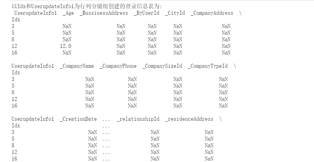
order3Pivot=pd.pivot_table(order3[['Idx','ListingInfo1','UserupdateInfo1','UserupdateInfo2']],index='Idx',columns='UserupdateInfo1',aggfunc=np.sum,fill_value=0)
print('with Idx and UserupdateInfo1 The information update table created for the row column sub key group is:\n',order3Pivot.head())

2. Use the crosstab method to convert long and wide tables

rder2Pivot=pd.crosstab(index=order2['Idx'],columns=order2['LogInfo1'],values=order2['LogInfo2'],aggfunc=np.sum)
print('with Idx and LogInfo1 The login information table created for the row column sub key group is:\n',order2Pivot.head())

order3Pivot=pd.crosstab(index=order3['Idx'],columns=order3['UserupdateInfo1'],values=order3['Idx'],aggfunc=np.sum)
print('with Idx and UserupdateInfo1 The login information table created for the row column sub key group is:\n',order3Pivot.head())