**Freight service network design: reading notes of classic literature (2) **It was mentioned that the model used in cranic T g (1984) should be reproduced, but the general framework given in the article is still too general. After trying, it was decided to use Netplan (1989) for LCL freight proposed by Jacques Roy & Louis Delorme on the basis of cranic T g (1984) as the blueprint of basic learning to realize the reproduction.
Netplan: A Network Optimization Model For Tactical Planning In The
Less-Than-Truckload Motor-Carrier Industry, INFOR: Information Systems and Operational Research, 27:1, 22-35, Jacques Roy & Louis Delorme (1989)
DOI: 10.1080/03155986.1989.11732079
I. overview of the paper
The deregulation of Canadian road freight market and fierce market competition have led to the emergence of netplan as a decision-making tool. Netplan originates from the general framework of freight service network design model and algorithm, and integrates the characteristics of medium and long-term planning of LCL freight service.
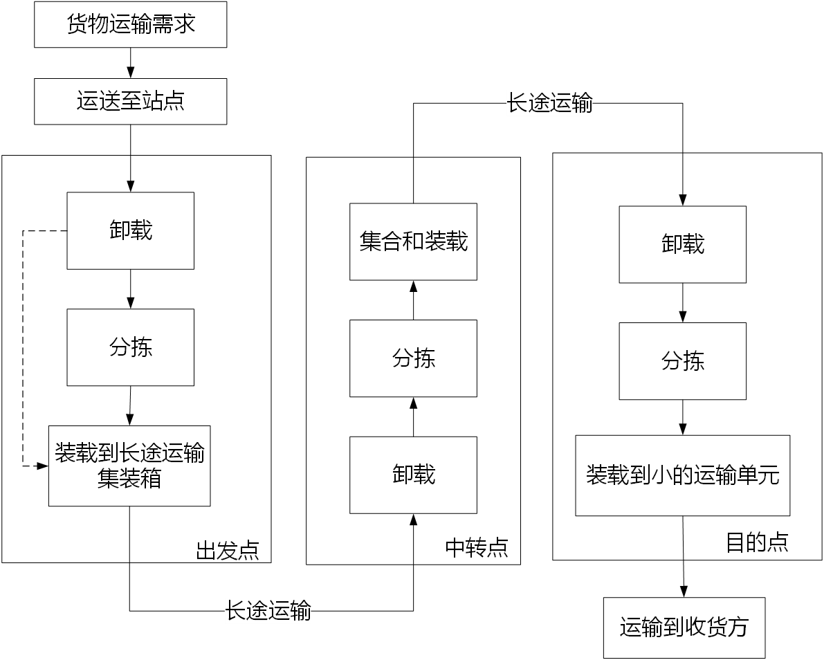
1.1 schematic diagram of less than carload freight business process
1.2 three problems in the design of LCL freight service network
Load Plan:
How to formulate the strategy of services between stations and transporting (separating and merging) goods on the network, so that the transportation strategy ensures to minimize the transportation and processing costs, while improving or at least maintaining the existing service level - Powell (1986)
The Load Plan must consider the following three interrelated sub problems:
- 1. Service Network Design, that is, select the route providing operator services and determine the characteristics of each service, such as mode, speed and frequency (vehicle departure times on a given route in each planning period)
- 2. The Traffic Distribution refers to which service sequence will be used to move the goods and which terminal the goods will pass through for each departure destination pair (or freight class) with positive freight demand
- 3. The Empty Vehicle Movement is to determine the number of empty vehicles required to move, so as to establish a balance between the number of departure vehicles and arrival vehicles at each originating terminal in the network
The third question is not explained in detail in the paper, so it is also ignored here for the time being.
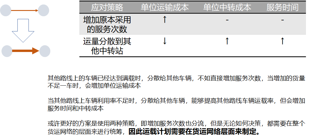
1.3 influence scope of freight network decision
Second, reproduce the thesis model
The main task of Netplan model is to help LCL freight enterprises make medium and long-term load plans at the freight network level. The language used is python, the solver uses gurobipy, and networkx for drawing
import sys
import math
import random
import gurobipy as gp
from gurobipy import GRB
from gurobipy import *
import numpy as np
import networkx as nx
import matplotlib.pyplot as plt
2.1 input data simulation
The first problem encountered in reproducing the paper is that there is no data, so all the data need to be simulated according to a certain logic. Now let's take a look at the data that will be used?
2.1.1 input data analysis
2.1.1.1 cost data
- intercity transportation costs: varies with the type of service used and its frequency
- the freight consolidation costs: varies with the volume of freight handled at the Breakbulk
- the capacity penalty costs: the penalty incurred when the trailer capacity is overused in each transportation service
- the service penalty costs: the penalty incurred when the service performance standard is not met, taking into account the average value and variance of the planned transportation time of each freight class
The relevant costs and cost units are listed above. Step by step, this paper only considers the first cost.
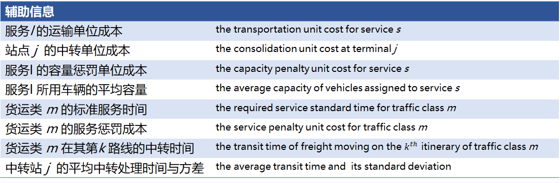
2.1.1.2 basic information
Here, the required information is listed first. Since a cost is considered first for the time being, some known information will not be used for the time being (so it does not need to be simulated this time)
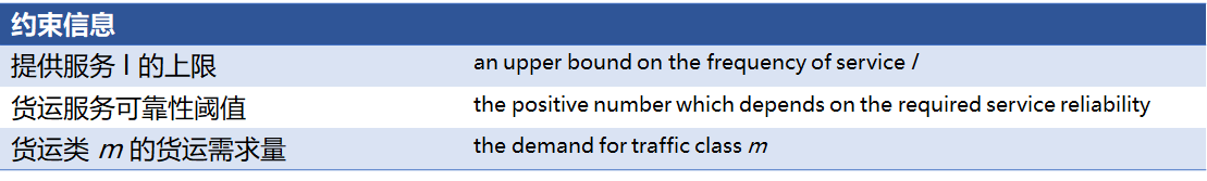
2.1.1.3 information to be decided
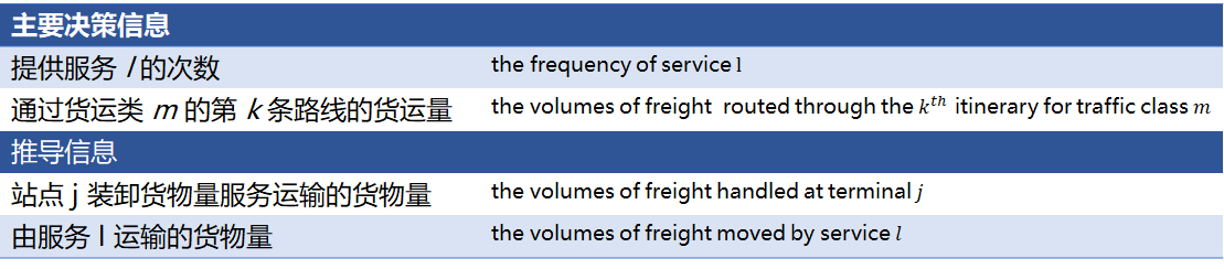
2.1.2 code generated by input data
# Example generation for the article NETPLAN(1989)
# Node set, number + coordinates

N = dict()
# Transit cost per node
Cn = dict()
for n in range(6):
    N.update({n:np.array([random.randint(0,20),random.randint(0,20)],dtype = np.float32)}) #Number + coordinates
    Cn.update({n:random.randint(5,10)}) # Transit cost per node

# Randomly generate the freight demand of OD pairs, and temporarily ignore the freight demand penalty and transportation time requirements
D = dict()
for i in range(30):
    o = random.randint(0,len(N)-1)
    d = random.randint(0,len(N)-1)
    while o == d:
        d = random.randint(0,len(N)-1)
    D.update({(o,d):random.randint(30,200)})
When I simulated here, I chose the idea of demand driven. Firstly, the set of less than carload freight demand is randomly generated. The freight demand is composed of OD pairs and corresponding freight volume, which is stored by dictionary type.
Therefore, in order to simplify the service path, only different service paths are defined. In this way, it is necessary to formulate path search rules, and before implementing these path search rules by program, it is necessary to determine the representation of the network.
The freight demand dictionary can also be regarded as a freight demand network, which is a directed network represented by an arc. [ps, edge generally refers to undirected connection, and arc refers to directed connection)
However, I don't think the network represented by arc is easy to use when searching the path, so I regenerate the dictionary type variable snet in the code. Its representation takes the node as the key and the node points to the node list as the value.
def find_degree(n, edges,out):
    '''
    Find the starting point in the graph represented by edge set n Point of arrival after departure
    Or arrival point n Starting point
    The Function is used to find the arriving node or
    the starting node for the node n in the net which is
    described by the edges set.
    thus parameter n indicates the node;
    edges is the net which is described by edges set;
    out indicates whether it is to find the arriving node (out =1)
    or the starting node (out =0).
    '''
    degree_n = []
    if out == 0:
        for i in edges:
            if n == i[0]:
                degree_n.append(i[1])
    else:
        for i in edges:
            if n == i[1]:
                degree_n.append(i[0])
    return degree_n

# Generate demand network
snet = dict()
for i in N.keys():
    deout = find_degree(i, D.keys(),0)
    snet.update({i:deout})
snet is used to generate services defined simply by paths
# Generate the service and the arc that the service passes through
L = dict()
#Service capacity
alpha = dict()
# Transportation unit cost of service
Cl = dict()
# Based on the demand network, generate the path passing through no more than two transit nodes, and then randomly generate the service capacity and service cost
k = 0
for o in range(len(N)):
    for d in range(o+1,len(N)):
        for l in searchGraph(snet, o, d): # More than 2 transit paths are not used
            # Triangle relation satisfying coordinates
            if len(l) == 3:
                l01 = ((N[l[0]][0] - N[l[1]][0])**2 + (N[l[0]][1] - N[l[1]][1])**2 )**0.5
                l02 = ((N[l[0]][0] - N[l[2]][0])**2 + (N[l[0]][1] - N[l[2]][1])**2 )**0.5
                l12 = ((N[l[1]][0] - N[l[2]][0])**2 + (N[l[1]][1] - N[l[2]][1])**2 )**0.5
                indicator = l01 + l12 > l02
                if indicator == True:
                    L.update({k:l})
                    Cl.update({k:random.randint(10,20)})
                    alpha.update({k:random.randint(2,4)*100})
                    k = k+1
            elif len(l) == 4:
                l01 = ((N[l[0]][0] - N[l[1]][0])**2 + (N[l[0]][1] - N[l[1]][1])**2 )**0.5
                l02 = ((N[l[0]][0] - N[l[2]][0])**2 + (N[l[0]][1] - N[l[2]][1])**2 )**0.5
                l03 = ((N[l[0]][0] - N[l[3]][0])**2 + (N[l[0]][1] - N[l[3]][1])**2 )**0.5
                l12 = ((N[l[1]][0] - N[l[2]][0])**2 + (N[l[1]][1] - N[l[2]][1])**2 )**0.5
                l13 = ((N[l[1]][0] - N[l[3]][0])**2 + (N[l[1]][1] - N[l[3]][1])**2 )**0.5
                l23 = ((N[l[2]][0] - N[l[3]][0])**2 + (N[l[2]][1] - N[l[3]][1])**2 )**0.5
                l03 = ((N[l[0]][0] - N[l[3]][0])**2 + (N[l[0]][1] - N[l[3]][1])**2 )**0.5

                ind1 = (l01 + l12) > l02
                ind2 = (l12 + l23) > l13
                ind3 = l03 > (l01+l12+l23)
                ind4
                ind5 = (l23 >= (0.3*(l01+l12+l23)))
                indicator1 = (ind1 & ind2 & ind3 & ind4)
                if indicator1 == True:
                    L.update({k:l})
                    Cl.update({k:random.randint(10,20)})
                    alpha.update({k:random.randint(2,4)*100})
                    k = k+1

            else:
                L.update({k:l})
                Cl.update({k:random.randint(10,20)})
                alpha.update({k:random.randint(2,4)*100})
                k = k+1
Although the code generated by the above service calculates the length of the path and maintains the triangular balance of the path, it will still generate a seemingly unreasonable path. However, because it is only simulation, we will temporarily give up the rules for further refining the path generation.
Therefore, more rules are needed in path generation to standardize the generated services. Of course, in practice, the service type is given by the freight enterprise, or it is also a small optimization problem (for example, the shortest path under different steps)
So far, the basic data can be simulated. The following is the further calculation on these data.
2.2 model data analysis
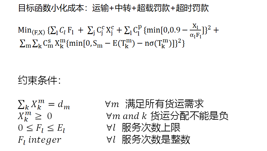
To learn step by step, this article only considers the transportation cost of using each service. One constraint is to allocate the freight volume in the service set that each freight class m can choose; The second constraint is that the freight volume cannot be negative. The third constraint is that the number of services is limited, a service can not be used, and the number of services is an integer. It can be found that except the first constraint, other constraints are constraints on the value range of decision variables, which can be realized directly in the function defining decision variables in programming.
Here is the code for Gurobipy to build the model.
# model building
Model = gp.Model('fsnd')

# Add variable

# Frequency of service l
F_l = Model.addVars(L,lb=0, vtype =GRB.INTEGER, name='Fre')

#Traffic volume on alternative route k of each freight flow m
X_mk = dict()
for m in m_path:
    for k in m_path[m]:
        X_mk[m,k] = Model.addVar(lb=0,vtype =GRB.INTEGER,name=f'x_{m}{k}')

# Minimize transportation costs
objective = Model.setObjective(gp.quicksum(F_l[l] * Cl[l] for l in L),GRB.MINIMIZE)

# Add constraint
# For any freight class m, the total transportation volume on k routes is equal to the transportation demand
i = 0
for m in m_path:
    Model.addConstr(gp.quicksum(X_mk[m,k] for k in m_path[m].keys())== D[m],name=f'C{i}')
    i = i + 1

# For any service, the number of times should be greater than the required transportation volume
for l in L:
    Model.addConstr(gp.quicksum(X_mk[m,l] for m in l_mset[l])<=F_l[l]*alpha[l], name=f'C{i}')
    i = i + 1

Model.optimize()

# Model error checking
if Model.status == GRB.Status.INFEASIBLE:
        print('Optimization was stopped with status %d' % Model.status)
        # do IIS, find infeasible constraints
        Model.computeIIS()
        for c in Model.getConstrs():
            if c.IISConstr:
                print('%s' % c.constrName)
In the generation of decision variables, it is worth mentioning that in fact, the number of alternative services of each freight class is different. Before building the model, it is necessary to screen out the set of alternative services of each freight class m.
# Optional service l set for each freight demand
m_path = dict()
for m in D:
    path = dict()
    for l in L:
        o_ind = findindex(m[0],L[l])
        d_ind = findindex(m[1],L[l])
        if 0 <= o_ind < d_ind:
            path.update({l:L[l]})
    m_path.update({m:path})
The constraint of this model actually restricts the number of services in the overload penalty cost of the objective function X l α l F l \frac{X_l}{\alpha_l F_l} α lFlXl. there X l X_l Xl , is an intermediate variable, because I don't consider the cost of overload here, so I add this constraint to the code implementation
If you write a formula
∑
m
∈
M
(
l
)
X
k
m
<
=
F
l
α
l
∀
l
\sum_{m \in M(l)}{X^m_k } <=F_l\alpha_l \quad \forall l
∑m∈M(l)Xkm<=Flαl∀l
X
l
=
∑
m
∈
M
(
l
)
X
k
m
∀
l
X_l = \sum_{m \in M(l)}{X^m_k } \quad \forall l
Xl=∑m∈M(l)Xkm∀l
M
(
l
)
M(l)
M(l) is the set of freight classes m applicable to each freight service l.
The following is the generation M ( l ) M(l) Code of M(l)
# For each service l, the freight class m set of possible services
l_mset = dict()
for l in L:
    mdict = dict()
    for m in m_path:
        if l in m_path[m].keys():
            mdict.update({m:0})
    l_mset.update({l:mdict})
Code corresponding to constraint
# For any service, the number of times should be greater than the required transportation volume
for l in L:
    Model.addConstr(gp.quicksum(X_mk[m,l] for m in l_mset[l])<=F_l[l]*alpha[l], name=f'C{i}')
    i = i + 1
2.3 data output
The data output part is mainly to visualize the results of gurobi solution.
Here is a log of one-time examples
Gurobi Optimizer version 9.1.1 build v9.1.1rc0 (win64)
Thread count: 4 physical cores, 8 logical processors, using up to 8 threads
Optimize a model with 76 rows, 259 columns and 458 nonzeros
Model fingerprint: 0x6b2ec18d
Variable types: 0 continuous, 259 integer (0 binary)
Coefficient statistics:
  Matrix range     [1e+00, 4e+02]
  Objective range  [1e+01, 2e+01]
  Bounds range     [0e+00, 0e+00]
  RHS range        [8e+01, 2e+02]
Found heuristic solution: objective 218.0000000
Presolve time: 0.00s
Presolved: 76 rows, 259 columns, 458 nonzeros
Variable types: 0 continuous, 259 integer (17 binary)

Root relaxation: objective 6.456032e+01, 131 iterations, 0.00 seconds

    Nodes    |    Current Node    |     Objective Bounds      |     Work
 Expl Unexpl |  Obj  Depth IntInf | Incumbent    BestBd   Gap | It/Node Time

     0     0   64.56032    0    9  218.00000   64.56032  70.4%     -    0s
H    0     0                     121.0000000   64.56032  46.6%     -    0s
H    0     0                     111.0000000   64.56032  41.8%     -    0s
H    0     0                      98.0000000   64.56032  34.1%     -    0s
H    0     0                      95.0000000   64.56032  32.0%     -    0s
H    0     0                      92.0000000   64.56032  29.8%     -    0s
     0     0   68.23180    0   21   92.00000   68.23180  25.8%     -    0s
H    0     0                      77.0000000   68.23180  11.4%     -    0s
     0     0   68.37794    0   19   77.00000   68.37794  11.2%     -    0s
     0     0   68.38825    0   25   77.00000   68.38825  11.2%     -    0s
     0     0   70.02606    0   18   77.00000   70.02606  9.06%     -    0s
     0     0   70.02606    0    8   77.00000   70.02606  9.06%     -    0s
     0     0   70.02606    0   11   77.00000   70.02606  9.06%     -    0s
     0     0   70.02606    0   21   77.00000   70.02606  9.06%     -    0s
     0     0   70.09949    0   18   77.00000   70.09949  8.96%     -    0s
     0     0   71.47247    0   31   77.00000   71.47247  7.18%     -    0s
     0     0   71.47286    0   31   77.00000   71.47286  7.18%     -    0s
     0     0   71.62734    0   18   77.00000   71.62734  6.98%     -    0s
     0     0   71.66762    0   38   77.00000   71.66762  6.93%     -    0s
     0     0   71.68363    0   38   77.00000   71.68363  6.90%     -    0s
H    0     0                      76.0000000   71.68363  5.68%     -    0s
     0     0   71.71158    0   15   76.00000   71.71158  5.64%     -    0s
     0     0   71.71158    0   19   76.00000   71.71158  5.64%     -    0s
     0     0   71.74907    0   45   76.00000   71.74907  5.59%     -    0s
     0     0   71.81435    0   28   76.00000   71.81435  5.51%     -    0s
H    0     0                      74.0000000   71.81435  2.95%     -    0s
     0     0   72.17717    0   24   74.00000   72.17717  2.46%     -    0s
     0     0   72.17717    0   19   74.00000   72.17717  2.46%     -    0s
     0     0   72.17717    0    8   74.00000   72.17717  2.46%     -    0s
     0     0   72.17717    0   17   74.00000   72.17717  2.46%     -    0s
     0     0   72.63333    0   22   74.00000   72.63333  1.85%     -    0s
     0     0   73.18750    0   26   74.00000   73.18750  1.10%     -    0s

Cutting planes:
  Gomory: 3
  MIR: 13
  Relax-and-lift: 2

Explored 1 nodes (554 simplex iterations) in 0.13 seconds
Thread count was 8 (of 8 available processors)

Solution count 9: 74 76 77 ... 218

Optimal solution found (tolerance 1.00e-04)
Best objective 7.400000000000e+01, best bound 7.400000000000e+01, gap 0.0000%
Output results
Freight (2, 0)_ 58: 81.0:[4, 2, 0, 5]
Freight (1, 4)_ 15: 41.0:[1, 0, 4, 2]
Freight (1, 4)_ 19: 39.0:[1, 4, 2, 3]
Freight (1, 4)_ 30: 109.0:[1, 3, 4, 5]
Freight (4, 2)_ 15: 189.0:[1, 0, 4, 2]
Freight (1, 0)_ 15: 149.0:[1, 0, 4, 2]
Freight (1, 3)_ 19: 94.0:[1, 4, 2, 3]
Freight (5, 2)_ 4: 100.0:[0, 4, 5, 2]
Freight (2, 5)_ 54: 78.0:[3, 2, 1, 5]
Freight (0, 4)_ 4: 188.0:[0, 4, 5, 2]
Freight (2, 3)_ 19: 167.0:[1, 4, 2, 3]
Freight (4, 5)_ 4: 64.0:[0, 4, 5, 2]
Freight (4, 5)_ 30: 23.0:[1, 3, 4, 5]
Freight (0, 5)_ 4: 48.0:[0, 4, 5, 2]
Freight (0, 5)_ 58: 58.0:[4, 2, 0, 5]
Freight (4, 0)_ 58: 161.0:[4, 2, 0, 5]
Freight (1, 5)_ 30: 73.0:[1, 3, 4, 5]
Freight (1, 5)_ 54: 54.0:[3, 2, 1, 5]
Freight (3, 4)_ 30: 195.0:[1, 3, 4, 5]
Freight (2, 1)_ 54: 88.0:[3, 2, 1, 5]
Freight (3, 2)_ 54: 180.0:[3, 2, 1, 5]
Service number: 4, service path: [0, 4, 5, 2], service capacity: 400, service times: 1.0, service freight volume: 49
Service number: 15, service path: [1, 0, 4, 2], service capacity: 400, service times: 1.0, service freight volume: 53
Service number: 19, service path: [1, 4, 2, 3], service capacity: 300, service times: 1.0, service freight volume: 45
Service number: 30, service path: [1, 3, 4, 5], service capacity: 400, service times: 1.0, service freight volume: 61
Service number: 54, service path: [3, 2, 1, 5], service capacity: 400, service times: 1.0, service freight volume: 48
Service number: 58, service path: [4, 2, 0, 5], service capacity: 300, service times: 1.0, service freight volume: 35
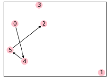
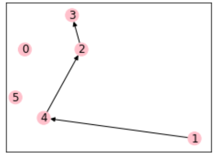
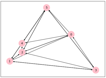
Network visualization before and after one optimization (independent of the above text results)
Optimize the first 21 service demand arcs
The optimized 12 service demand arcs reduce the cost by combining the freight demand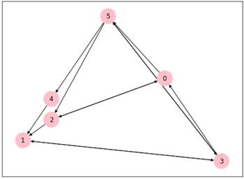
Detail 1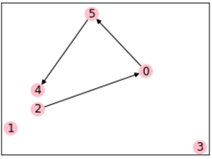
Detail 2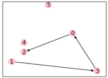
It can be seen that the freight demand is indeed consolidated, which can also explain why sometimes our express will first detour and then be transported. This is just that the freight company is saving costs. Of course, if the service time is considered, the result will be different.