1, Introduction

Alex net was designed by Hinton, the winner of the 2012 ImageNet competition, and his student Alex Krizhevsky. Also after that year, more and deeper neural networks were proposed, such as the excellent VGg and Google lenet. The accuracy of the official data model is 57.1% and the top 1-5 is 80.2%. This is quite excellent for the traditional machine learning classification algorithm.

2, Network structure

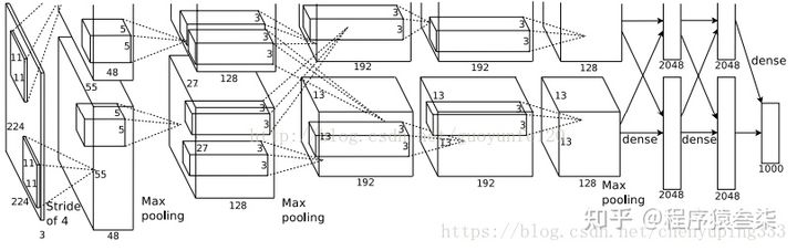
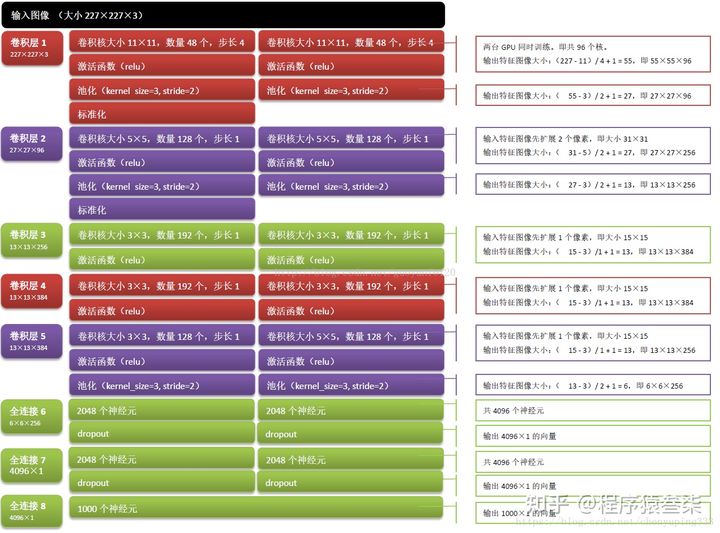
The figure above shows the network structure of alexnet in caffe. The figure above shows two GPU servers. You can see two flow charts. The network structure of alexnet is shown below:

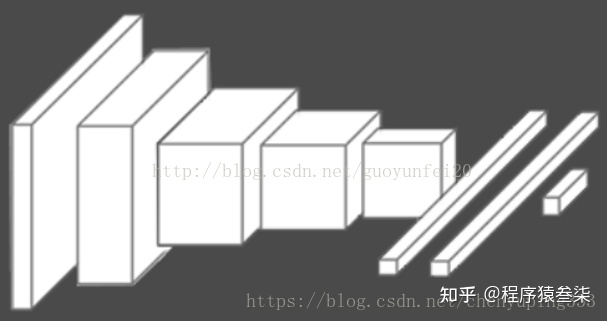
The simplified structure is:

Why did AlexNet achieve better results?

1. The Relu activation function is used.

Relu function: f(x)=max(0,x)

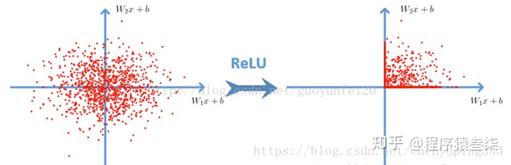
The deep convolution network based on ReLU is several times faster than the network based on tanh and sigmoid. The following figure shows the number of iterations of a four-layer convolution network based on CIFAR-10 with 25% training error in tanh and ReLU;

2. Local Response Normalization

After using ReLU f(x)=max(0,x), you will find that the value after the activation function does not have a value range like tanh and sigmoid functions. Therefore, generally, a normalization will be done after ReLU. LRU is a method that is steadily proposed (uncertain here, it should be proposed?). In neuroscience, there is a concept called "late inhibition", It's about the effect of active neurons on their peripheral neurons.

3. Dropout

Dropout is also a frequently mentioned concept, which can effectively prevent over fitting of neural network. Compared with the general linear model, the regular method is used to prevent the model from over fitting, while in the neural network, dropout is realized by modifying the structure of the neural network itself. For a certain layer of neurons, some neurons are deleted randomly through the defined probability, while keeping the individuals of neurons in the input layer and output layer unchanged, and then the parameters are updated according to the learning method of neural network. In the next iteration, some neurons are deleted randomly again until the end of training.

4. data augmentation

In deep learning, when the amount of data is not large enough, there are generally four solutions:

• data augmentation - manually increase the size of the training set - create a batch of "new" data from the existing data by translating, flipping, adding noise and other methods
• Regularization - a small amount of data will lead to over fitting of the model, making the training error very small and the test error particularly large. The generation of over fitting can be suppressed by adding a regular term after the Loss Function. The disadvantage is the introduction of a hyper parameter that needs to be adjusted manually.
• Dropout is also a regularization method, but different from the above, it is realized by randomly setting the output of some neurons to zero
• Unsupervised pre training -- unsupervised pre training is performed layer by layer in the convolution form of auto encoder or RBM, and finally supervised fine tuning is performed with the classification layer

3, tensorflow code implementation

# -*- coding=UTF-8 -*-
import sys
import os
import random
import cv2
import math
import time
import numpy as np
import tensorflow as tf
import linecache
import string
import skimage
import imageio
# input data
import input_data
mnist = input_data.read_data_sets("/tmp/data/", one_hot=True)
# Define network superparameters
learning_rate = 0.001
training_iters = 200000
batch_size = 64
display_step = 20
# Define network parameters
n_input = 784  # Dimension entered
n_classes = 10 # Dimension of label
dropout = 0.8  # Dropout probability
# Placeholder input
x = tf.placeholder(tf.types.float32, [None, n_input])
y = tf.placeholder(tf.types.float32, [None, n_classes])
keep_prob = tf.placeholder(tf.types.float32)
# Convolution operation
def conv2d(name, l_input, w, b):
    return tf.nn.relu(tf.nn.bias_add( \
    tf.nn.conv2d(l_input, w, strides=[1, 1, 1, 1], padding='SAME'),b) \
    , name=name)
# Maximum downsampling operation
def max_pool(name, l_input, k):
    return tf.nn.max_pool(l_input, ksize=[1, k, k, 1], \
    strides=[1, k, k, 1], padding='SAME', name=name)
# Normalization operation
def norm(name, l_input, lsize=4):
    return tf.nn.lrn(l_input, lsize, bias=1.0, alpha=0.001 / 9.0, beta=0.75, name=name)
# Define the entire network 
def alex_net(_X, _weights, _biases, _dropout):
    _X = tf.reshape(_X, shape=[-1, 28, 28, 1]) # Vector to matrix
    # Convolution layer
    conv1 = conv2d('conv1', _X, _weights['wc1'], _biases['bc1'])
    # Lower sampling layer
    pool1 = max_pool('pool1', conv1, k=2)
    # Normalization layer
    norm1 = norm('norm1', pool1, lsize=4)
    # Dropout
    norm1 = tf.nn.dropout(norm1, _dropout)
 
    # convolution
    conv2 = conv2d('conv2', norm1, _weights['wc2'], _biases['bc2'])
    # Down sampling
    pool2 = max_pool('pool2', conv2, k=2)
    # normalization
    norm2 = norm('norm2', pool2, lsize=4)
    # Dropout
    norm2 = tf.nn.dropout(norm2, _dropout)
 
    # convolution
    conv3 = conv2d('conv3', norm2, _weights['wc3'], _biases['bc3'])
    # Down sampling
    pool3 = max_pool('pool3', conv3, k=2)
    # normalization
    norm3 = norm('norm3', pool3, lsize=4)
    # Dropout
    norm3 = tf.nn.dropout(norm3, _dropout)
 
    # In the full connection layer, first turn the characteristic graph into a vector
    dense1 = tf.reshape(norm3, [-1, _weights['wd1'].get_shape().as_list()[0]]) 
    dense1 = tf.nn.relu(tf.matmul(dense1, _weights['wd1']) + _biases['bd1'], name='fc1') 
    # Full connection layer
    dense2 = tf.nn.relu(tf.matmul(dense1, _weights['wd2']) + _biases['bd2'], name='fc2') # Relu activation
 
    # Network output layer
    out = tf.matmul(dense2, _weights['out']) + _biases['out']
    return out
 
# Store all network parameters
weights = {
    'wc1': tf.Variable(tf.random_normal([3, 3, 1, 64])),
    'wc2': tf.Variable(tf.random_normal([3, 3, 64, 128])),
    'wc3': tf.Variable(tf.random_normal([3, 3, 128, 256])),
    'wd1': tf.Variable(tf.random_normal([4*4*256, 1024])),
    'wd2': tf.Variable(tf.random_normal([1024, 1024])),
    'out': tf.Variable(tf.random_normal([1024, 10]))
}
biases = {
    'bc1': tf.Variable(tf.random_normal([64])),
    'bc2': tf.Variable(tf.random_normal([128])),
    'bc3': tf.Variable(tf.random_normal([256])),
    'bd1': tf.Variable(tf.random_normal([1024])),
    'bd2': tf.Variable(tf.random_normal([1024])),
    'out': tf.Variable(tf.random_normal([n_classes]))
}
# Build model
pred = alex_net(x, weights, biases, keep_prob)
# Define loss function and learning steps
cost = tf.reduce_mean(tf.nn.softmax_cross_entropy_with_logits(pred, y))
optimizer = tf.train.AdamOptimizer(learning_rate=learning_rate).minimize(cost)
# Test network
correct_pred = tf.equal(tf.argmax(pred,1), tf.argmax(y,1))
accuracy = tf.reduce_mean(tf.cast(correct_pred, tf.float32))
# Initialize all shared variables
init = tf.initialize_all_variables()
# Start a workout
with tf.Session() as sess:
    sess.run(init)
    step = 1
    # Keep training until reach max iterations
    while step * batch_size < training_iters:
        batch_xs, batch_ys = mnist.train.next_batch(batch_size)
        # Get batch data
        sess.run(optimizer, feed_dict={x: batch_xs, y: batch_ys, keep_prob: dropout})
        if step % display_step == 0:
            # Calculation accuracy
            acc = sess.run(accuracy, feed_dict={x: batch_xs, y: batch_ys, keep_prob: 1.})
            # Calculate loss value
            loss = sess.run(cost, feed_dict={x: batch_xs, y: batch_ys, keep_prob: 1.})
            print "Iter " + str(step*batch_size) + ", Minibatch Loss= " + "{:.6f}".format(loss) + ", Training Accuracy= " + "{:.5f}".format(acc)
        step += 1
    print "Optimization Finished!"
    # Calculate test accuracy
    print "Testing Accuracy:", sess.run(accuracy, feed_dict={x: mnist.test.images[:256], y: m