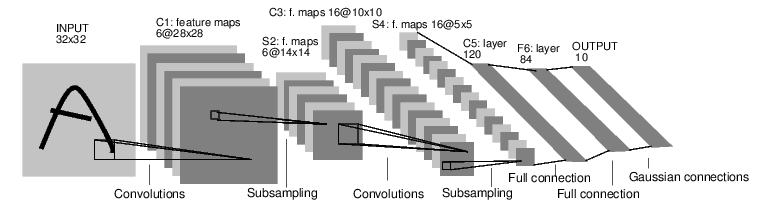
The figure above shows the architecture of the LeNet-5 model.
It was proposed by Professor Yann LeCun in his paper "graduate based learning applied to document recognition" in 1998. It is the first convolutional neural network successfully applied to digital recognition.
LeNet-5 detailed structure
The structure of each layer of the LeNet-5 model will be described in detail in the following pages.
First layer, convolution layer
The input of this layer is the original image pixels, and the input layer size accepted by LeNet-5 model is 32 × thirty-two × 1. The size of the first convolution filter is 5 × 5. The depth is 6, full 0 filling is not used, and the step is 1. Because full 0 filling is not used, the output size of this layer is 32 − 5 + 1 = 28 and the depth is 6. There are a total of 5 in this convolution × five × one × 6 + 6 = 156 parameters, of which 6 are offset term parameters. Because the node matrix of the next layer has 28 × twenty-eight × 6 = 4704 nodes, 5 for each node × 5 = 25 nodes of the current layer are connected, so there are 4704 convolution layers in this layer × (25 + 1) = 122304 connections.
Second floor, pool layer
The input of this layer is the output of the first layer, which is a 28 × twenty-eight × 6 node matrix. The filter size used in this layer is 2 × 2. The steps of length and width are both 2, so the output matrix size of this layer is 14 × fourteen × 6.
Third layer, convolution layer
The input matrix size of this layer is 14 × fourteen × 6. The filter size used is 5 × 5. The depth is 16. This layer does not use full 0 filling, and the step is 1. The output matrix size of this layer is 10 × ten × 16. According to the standard convolution layer, this layer should have 5 × five × six × 16 + 16 = 2416 parameters, 10 × ten × sixteen × (25 + 1) = 41600 connections.
The fourth layer, pool layer
The input matrix size of this layer is 10 × ten × 16. The filter size adopted is 2 × 2. The step is 2. The output matrix size of this layer is 5 × five × 16.
Fifth floor, full connection floor
The input matrix size of this layer is 5 × five × 16. In the paper of LeNet-5 model, this layer is called convolution layer, but because the size of the filter is 5 × 5. Therefore, it is no different from the full connection layer. This layer will also be regarded as the full connection layer in the implementation of TensorFlow program. If 5 × five × 16. If the nodes in the matrix are pulled into a vector, the input of this layer is the same as that of the full connection layer. The number of output nodes in this layer is 120, with a total of 5 × five × sixteen × 120 + 120 = 48120 parameters.
Sixth floor, full connection floor
There are 120 input nodes and 84 output nodes in this layer, with a total of 120 parameters × 84 + 84 = 10164.
Seventh floor, full connection floor
There are 84 input nodes and 10 output nodes in this layer, with a total of 84 parameters × 10 + 10 = 850.
TensorFlow implementation
# Adjust the format of the input data placeholder and input it as a four-dimensional matrix.
x = tf.placeholder(tf.float32, [
		BATCH_SIZE, # The first dimension represents the number of samples in a batch.
		mnist_inference.IMAGE_SIZE, # The second and third dimensions represent the size of the picture.
		mnist_inference.IMAGE_SIZE,
		mnist_inference.NUM_CHANNELS], # The fourth dimension represents the depth of the picture. For RBG lattice
		# A picture with a depth of 3.
	name='x-input')

# Similarly, adjust the input training data format to a four-dimensional matrix, and transfer the adjusted data to sess Run procedure.
reshaped_xs = np.reshape(xs, (BATCH_SIZE,
		mnist_inference.IMAGE_SIZE,
		mnist_inference.IMAGE_SIZE,
		mnist_inference.NUM_CHANNELS))
# -*- coding: utf-8 -*-
import tensorflow as tf

# Configure the parameters of the neural network.
INPUT_NODE = 784  # 28x28
OUTPUT_NODE = 10  # 10 classification
IMAGE_SIZE = 28   # Picture pixel size
NUM_CHANNELS = 1  # Grayscale image with depth of 1
NUM_LABELS = 10   # Number of marks, 10 numbers

# The size and depth of the first layer of convolution.
CONV1_DEEP = 32
CONV1_SIZE = 5

# The size and depth of the second layer of convolution.
CONV2_DEEP = 64
CONV2_SIZE = 5

# Number of nodes in the full connection layer.
FC_SIZE = 512

# The forward propagation process of convolutional neural network is defined. A new parameter train is added here to distinguish between training process and test
# Process. dropout method will be used in this program. dropout can further improve the reliability of the model and prevent over fitting,
# The dropout procedure is used only during training.

def inference(input_tensor, train, regularizer):
    # Declare the variables of the first layer and realize the forward propagation process.
    # By using different namespaces to isolate variables in different layers, it can make the naming of variables in each layer only need
    # Consider the role in the current layer without worrying about the problem of duplicate names. Different from the standard LeNet-5 model, here
    # The defined convolution layer input is 28 × twenty-eight × 1 pixel of the original MNIST picture. Because all 0 filling is used in the convolution layer,
    # So the output is 28 × twenty-eight × 32 (CONV1_DEEP = 32).
    with tf.variable_scope('layer1-conv1'):
        conv1_weights = tf.get_variable(
            "weight", [CONV1_SIZE, CONV1_SIZE, NUM_CHANNELS, CONV1_DEEP],
            initializer=tf.truncated_normal_initializer(stddev=0.1))
        conv1_biases = tf.get_variable(
            "bias", [CONV1_DEEP], initializer=tf. constant_initializer(0.0))
        # Use a filter with a side length of 5 and a depth of 32. The filter moves in steps of 1 and is filled with all 0.
        conv1 = tf.nn.conv2d(
            input_tensor, conv1_weights, strides=[1, 1, 1, 1], padding='SAME')
        relu1 = tf.nn.relu(tf.nn.bias_add(conv1, conv1_biases))

# Realize the forward propagation process of the second pool layer. Here, the maximum pool layer is selected, and the side length of the pool layer filter is 2,
# Fill with all zeros and move in steps of 2. The input of this layer is the output of the previous layer, that is, 28 × twenty-eight × thirty-two
# Matrix of. The output is 14 × fourteen × 32 matrix.
with tf.name_scope('layer2-pool1'):
    pool1 = tf.nn.max_pool(
        relu1, ksize=[1, 2, 2, 1], strides=[1, 2, 2, 1], padding='SAME')

# Declare the variables of the third layer and realize the forward propagation process. The input of this layer is 14 × fourteen × 32 matrix.
# The output is 14 × fourteen × 64 matrix.
with tf.variable_scope('layer3-conv2'):
    conv2_weights = tf.get_variable(
        "weight", [CONV2_SIZE, CONV2_SIZE, CONV1_DEEP, CONV2_DEEP],
        initializer=tf.truncated_normal_initializer(stddev=0.1))
    conv2_biases = tf.get_variable(
        "bias", [CONV2_DEEP],
        initializer=tf. constant_initializer(0.0))
    # Use a filter with a side length of 5 and a depth of 64. The filter moves in steps of 1 and is filled with all 0.
    conv2 = tf.nn.conv2d(
        pool1, conv2_weights, strides=[1, 1, 1, 1], padding='SAME')
    relu2 = tf.nn.relu(tf.nn.bias_add(conv2, conv2_biases))

# Realize the forward propagation process of the fourth pool layer. The structure of this floor is the same as that of the second floor. The input of this layer is
# fourteen × fourteen × 64 matrix, output is 7 × seven × 64 matrix.
with tf.name_scope('layer4-pool2'):
    pool2 = tf.nn.max_pool(
        relu2, ksize=[1, 2, 2, 1], strides=[1, 2, 2, 1], padding='SAME')

# Convert the output of the fourth layer pooling layer into the input format of the fifth layer full connection layer. The output of the fourth layer is 7 × seven × 64 matrix,
# However, the input format required by the fifth layer full connection layer is vector, so this 7 is required here × seven × The matrix of 64 is straightened into one
# A vector. pool2. get_ The shape function can obtain the dimension of the fourth layer output matrix without manual calculation. be careful
# Because the input and output of each layer of neural network is a batch matrix, the dimension obtained here also includes a
# The number of data in batch.
pool_shape = pool2.get_shape().as_list()

# Calculate the length after straightening the matrix into a vector. This length is the product of the length, width and depth of the matrix. Pay attention here
# pool_shape[0] is the number of data in a batch.
nodes = pool_shape[1] * pool_shape[2] * pool_shape[3]

# Through TF The reshape function turns the output of the fourth layer into a batch vector.
reshaped = tf.reshape(pool2, [pool_shape[0], nodes])

# Declare the variables of the fifth layer and the whole connection layer, and realize the forward propagation process. The input of this layer is a set of vectors after straightening,
# The length of the vector is 3136, and the output is a set of vectors with a length of 512. This floor
# The concept of dropout is introduced. Dropout will randomly change the position of some nodes during training
# The output is changed to 0. dropout can avoid the over fitting problem, which makes the model better in the test data.
# [dropout is generally only used in the full connection layer rather than the convolution layer or pooling layer].
with tf.variable_scope('layer5-fc1'):
    fc1_weights = tf.get_variable(
        "weight", [nodes, FC_SIZE],
        initializer=tf.truncated_normal_initializer(stddev=0.1))

    # Only the weight of the whole connection layer needs to be regularized.
    if regularizer != None:
        tf.add_to_collection('losses', regularizer(fc1_weights))
    fc1_biases = tf.get_variable(
        "bias", [FC_SIZE], initializer=tf.constant_initializer(0.1))
    fc1 = tf.nn.relu(tf.matmul(reshaped, fc1_weights) + fc1_biases)
    if train: fc1 = tf.nn.dropout(fc1, 0.5)

# Declare the variables of the whole connection layer of the sixth layer and realize the forward propagation process. The input of this layer is a set of vectors with a length of 512,
# The output is a set of vectors with a length of 10. After the output of this layer passes through Softmax, the final classification result is obtained.
with tf.variable_scope('layer6-fc2'):
    fc2_weights = tf.get_variable(
        "weight", [FC_SIZE, NUM_LABELS],
        initializer=tf.truncated_normal_initializer(stddev=0.1))
    if regularizer != None:
        tf.add_to_collection('losses', regularizer(fc2_weights))
    fc2_biases = tf.get_variable(
        "bias", [NUM_LABELS],
        initializer=tf.constant_initializer(0.1))
    logit = tf.matmul(fc1, fc2_weights) + fc2_biases

# Returns the output of the sixth layer.
return logit
# Output results
$ python test.py
Extracting /tmp/data/train-images-idx3-ubyte.gz
Extracting /tmp/data/train-labels-idx1-ubyte.gz
Extracting /tmp/data/t10k-images-idx3-ubyte.gz
Extracting /tmp/data/t10k-labels-idx1-ubyte.gz
After 1 training step(s), loss on training batch is 6.45373.
After 1001 training step(s), loss on training batch is 0.824825.
After 2001 training step(s), loss on training batch is 0.646993.
After 3001 training step(s), loss on training batch is 0.759975.
After 4001 training step(s), loss on training batch is 0.68468.
After 5001 training step(s), loss on training batch is 0.630368.
How to design the architecture of convolutional neural network? The following regular expression formulas summarize some classical convolutional neural network architectures for image classification problems:
Input layer → (convolution layer + → pooling layer?)+ → full connection layer+
In the above formula, "convolution layer +" means one or more convolution layers. In most convolution neural networks, three convolution layers are usually used continuously at most.
"Pool layer?" Indicates that there is no or a pool layer. Although the pooling layer can reduce the parameters and prevent the over fitting problem, it is also found in some papers that it can be completed directly by adjusting the convolution step size. Therefore, some convolutional neural networks have no pooling layer. After multiple convolution layers and pooling layers, the convolutional neural network generally passes through 1 ~ 2 full connection layers before output.
For example, the LeNet-5 model can be expressed as the following structure.
Input layer → convolution layer → pooling layer → convolution layer → pooling layer → full connection layer → full connection layer → output layer
statement
This blog is an excerpt of some notes and feelings from personal learning, which is not guaranteed to be original. The content collects relevant online materials and secretary's content. There must be omissions and unmarked ones. If there is infringement, please contact the blogger.