Classic network VGG16

structure

According to the size of convolution kernel and the number of convolution layers, VGG can be divided into six configurations: A, a-lrn, B, C, D and E. among them, D and E are commonly used, which are called VGG16 and VGG19 respectively.

The following figure shows six structural configurations of VGG:

 

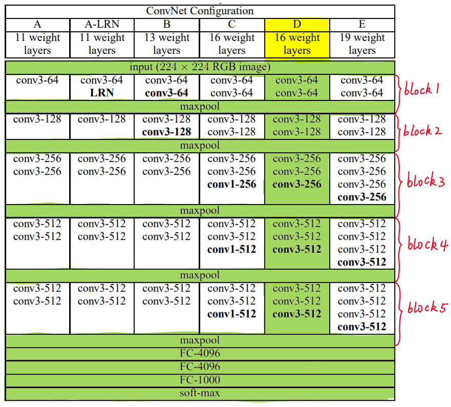
In the figure above, each column corresponds to a structure configuration. For example, the green part in the figure indicates the structure adopted by VGG16.

Through specific analysis of VGG16, we found that VGG16 includes:

• 13 convolutional layers, represented by conv3 XXX respectively
• Three fully connected layers are represented by FC-XXXX respectively
• Five pool layers are represented by maxpool

Among them, the convolution layer and the full connection layer have weight coefficients, so they are also called weight layers. The total number is 13 + 3 = 16, which is

Source of 16 in VGG16. (the pooling layer does not involve weight, so it does not belong to the weight layer and is not counted).

characteristic

The outstanding feature of VGG16 is simplicity, which is reflected in:

1. The convolution layers adopt the same convolution kernel parameters

   The convolution layers are expressed as conv3 XXX, where conv3 indicates that the size of the convolution core used in the convolution layer is 3, that is, the width and height are 3, and 3 * 3 is a very small convolution core size. Combined with other parameters (step stripe = 1, padding=same), In this way, each convolution layer (tensor) can maintain the same width and height as the previous layer (tensor). XXX represents the number of channels of the convolution layer.

2. The pool layer adopts the same pool core parameters

   The parameters of pool layer are 2 ×× 2. Pool mode with stride stripe = 2 and max, so that the width and height of each pool layer (tensor) are 1212 of the previous layer (tensor).

3. The model is composed of several convolution layers and pool layer stack ing, which is easy to form a deeper network structure (in 2014, 16 layers have been considered to be very deep).

Based on the above analysis, the advantages of VGG can be summarized as: small filters, deep networks

 

Block structure

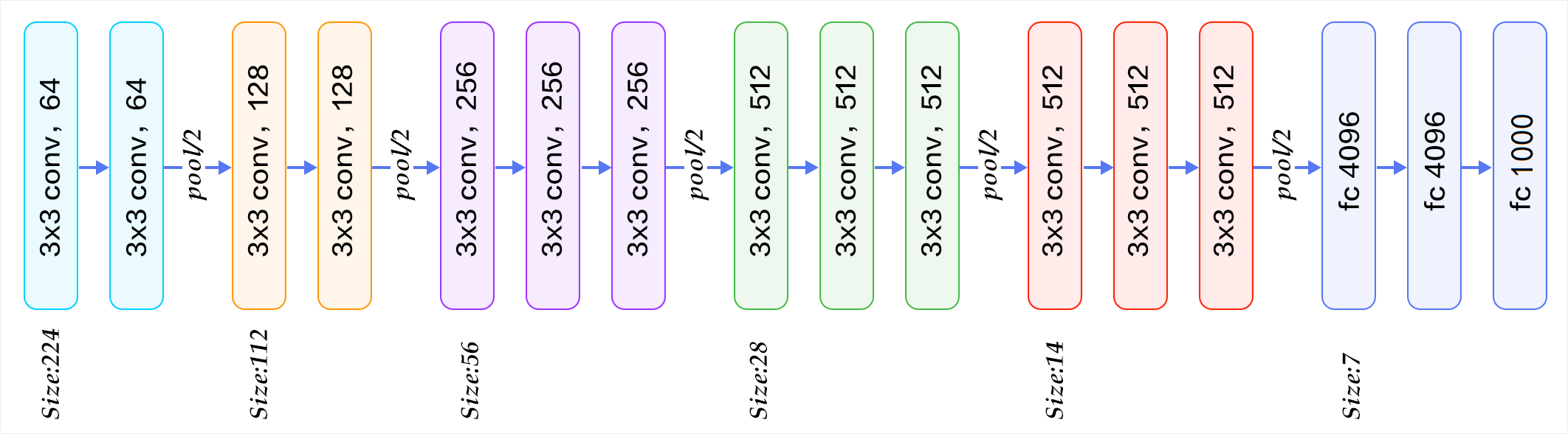
On the right side of Figure 1, the convolution layer and pooling layer of VGG16 can be divided into different blocks, which are numbered as Block1~block5 from front to back. Each Block contains several convolution layers and a pool layer. For example: Block4 contains:

• 3 convolution layers, conv3-512
• 1 pool layer, maxpool

And the number of channel s in the convolution layer is the same in the same block, for example:

• block2 contains two convolution layers. Each convolution layer is represented by conv3-128, that is, the convolution core is 3x3x3 and the number of channels is 128
• block3 contains three convolution layers, and each convolution layer is represented by conv3-256, that is, the convolution core is 3x3x3, and the number of channels is 256

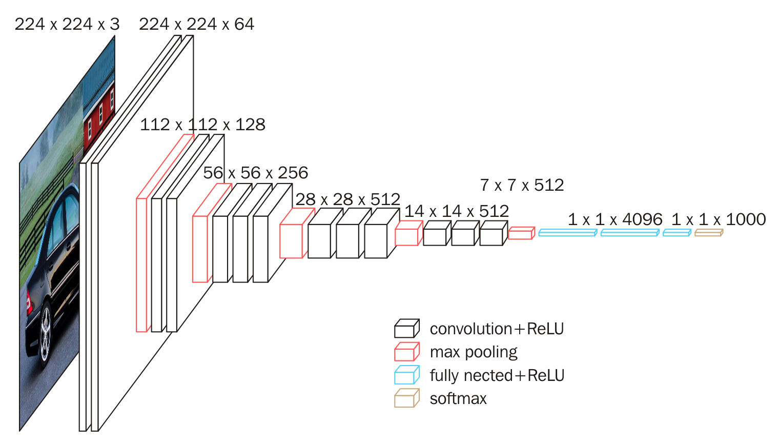
The structure diagram of VGG16 divided by blocks is given below, which can be understood in combination with figure 2:

 

The input image of VGG is a 224x224x3 image tensor. With the increase of the number of layers, the tensor in the latter block is compared with that in the previous block:

• The number of channels is doubled, from 64 to 128, then to 256, until 512 remains unchanged and does not double
• The height and width are halved, from 224 → 112 → 56 → 28 → 14 → 7

Weight parameter

Although the structure of VGG is simple, it contains a large number of weights, reaching an amazing 139357544 parameters. These parameters include convolution kernel weight and full connection layer weight.

• For example, for the first layer convolution, since the number of channels of the input graph is 3, the network must learn a convolution kernel with a size of 3x3 and a number of channels of 3. There are 64 such convolution kernels, so there are a total of (3x3x3) x64 = 1728 parameters

• The method for calculating the number of weight parameters of the full connection layer is: the number of nodes in the previous layer × Number of nodes in this layer number of nodes in the previous layer × Number of nodes in this layer. Therefore, the parameters of the whole connection layer are:

• • 7x7x512x4096 = 1027,645,444
  • 4096x4096 = 16,781,321
  • 4096x1000 = 4096000

code

def vgg16(input_shape=(224, 224, 3), classes=20):
    inputs = Input(shape=input_shape)                                                               # (224, 224, 3)
    x = layers.Conv2D(64, kernel_size=3, strides=1, padding='same', activation='relu')(inputs)      # (224, 224, 64)
    x = layers.Conv2D(64, kernel_size=3, strides=1, padding='same', activation='relu')(x)           # (224, 224, 64)
    x = layers.MaxPool2D(pool_size=(2, 2), strides=2)(x)                                            # (112, 112, 64)
    x = layers.Conv2D(128, kernel_size=3, strides=1, padding='same', activation='relu')(x)          # (112, 112, 128)
    x = layers.Conv2D(128, kernel_size=3, strides=1, padding='same', activation='relu')(x)          # (112, 112, 128)
    x = layers.MaxPool2D(pool_size=(2, 2), strides=2)(x)                                            # (56, 56, 128)
    x = layers.Conv2D(256, kernel_size=3, strides=1, padding='same', activation='relu')(x)          # (56, 56, 256)
    x = layers.Conv2D(256, kernel_size=3, strides=1, padding='same', activation='relu')(x)          # (56, 56, 256)
    x = layers.Conv2D(256, kernel_size=1, strides=1, padding='same', activation='relu')(x)          # (56, 56, 256)
    x = layers.MaxPool2D(pool_size=(2, 2), strides=2)(x)                                            # (28, 28, 256)
    x = layers.Conv2D(512, kernel_size=3, strides=1, padding='same', activation='relu')(x)          # (28, 28, 512)
    x = layers.Conv2D(512, kernel_size=3, strides=1, padding='same', activation='relu')(x)          # (28, 28, 512)
    x = layers.Conv2D(512, kernel_size=1, strides=1, padding='same', activation='relu')(x)          # (28, 28, 512)
    x = layers.MaxPool2D(pool_size=(2, 2), strides=2)(x)                                            # (14, 14, 512)
    x = layers.Conv2D(512, kernel_size=3, strides=1, padding='same', activation='relu')(x)          # (14, 14, 512)
    x = layers.Conv2D(512, kernel_size=3, strides=1, padding='same', activation='relu')(x)          # (14, 14, 512)
    x = layers.Conv2D(512, kernel_size=1, strides=1, padding='same', activation='relu')(x)          # (14, 14, 512)
    x = layers.MaxPool2D(pool_size=(2, 2), strides=2)(x)                                            # (7, 7, 512)
    x = layers.Flatten()(x)                                                                         # (7*7*512)
    x = layers.Dropout(rate=0.5)(x)
    x = layers.Dense(4096)(x)                                                                       # (4096)
    x = layers.Dropout(rate=0.5)(x)
    x = layers.Dense(4096)(x)                                                                       # (4096)
    x = layers.Dense(classes)(x)                                                                    # (classes)
    outputs = layers.Softmax()(x)
    model = Model(inputs, outputs)
    return model