Prepare training and test data sets
As soon as I came up, I found that the dataset could not be found. After searching, I finally found the dataset in another package.
# install.packages("C50")
# library(C50)
# data('churn', package = 'C50')
# install.packages("modeldata")
# https://stackoverflow.com/questions/60506936/data-set-churn-not-found-in-package-c50
library(modeldata)
data(mlc_churn)
churn <- mlc_churn
# 7: 3-point training and test set
set.seed(2)
ind <- sample(2,nrow(churnTrain),replace = TRUE,
              prob = c(0.7,0.3))
trainset <- churnTrain[ind==1,]
testset <- churnTrain[ind==2,]
This data set is slightly different from that in the book, but it should contain more relationships. There are more samples of this data, which should not be affected. Extension: split function completes the division of training and testing
split.data <- function(data, p= 0.7, s= 666){
  set.seed(s)
  index <- sample(1:dim(data)[1])
  train <- data[index[1:floor(dim(data)[1]*p)],]
  test <-  data[index[((ceiling(dim(data)[1]*p))+1):dim(data)[1]],]
  return(list(train=train,test=test))
}

li <- split.data(churnTrain)
Using recursive segmentation tree to establish classification model
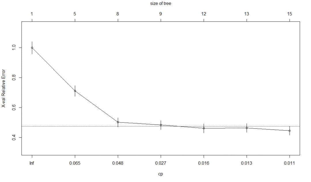
Recursion and segmentation are two steps of this algorithm. CP is a cost complexity parameter. The disadvantage of decision tree algorithm is that it is easy to produce deviation and over adaptation. Conditional reasoning tree can overcome deviation, and over adaptation can be solved by random forest method or tree pruning.
library(rpart)
churn.rp <- rpart(churn~., data=trainset)
plotcp(churn.rp)
summary(churn.rp)
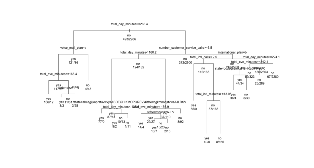
5.4 recursive split tree visualization
plot and text functions draw a classification tree.
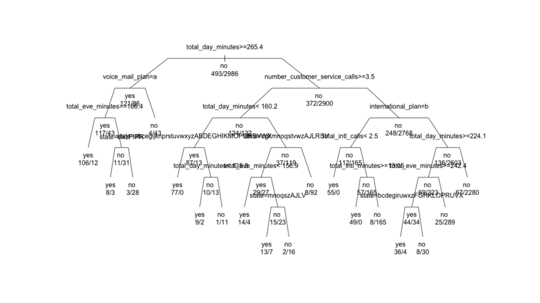
plot(churn.rp, margin = 0.1) # frame
text(churn.rp, all = TRUE, use.n = TRUE) # use.n number of actual observations per category
# Change the parameters to adjust the display results
plot(churn.rp, uniform = TRUE, branch = 0.6, margin = 0.1) # brach setting shoudler
text(churn.rp,all = TRUE, use.n = TRUE)
5.5 evaluate the classification ability of recursive split tree
# forecast
predictions <- predict(churn.rp, testset, type = "class")
table(testset$churn, predictions)
# #############
     predictions
       yes   no
  yes  133   81
  no    29 1278
# Generating confusion matrix
library(caret)
confusionMatrix(table(predictions, testset$churn))
Confusion Matrix and Statistics
# ##############

predictions  yes   no
        yes  133   29
        no    81 1278

               Accuracy : 0.9277
                 95% CI : (0.9135, 0.9402)
    No Information Rate : 0.8593
    P-Value [Acc > NIR] : < 2.2e-16

                  Kappa : 0.6671
5.6 recursive split tree pruning
Sometimes, it is necessary to prune the rules with weak classification description ability to avoid over adaptation and improve the prediction accuracy. The cost complexity method is used here.
min(churn.rp$cptable[,"xerror"])
[1] 0.4523327
which.min(churn.rp$cptable[,"xerror"])
5
5
# Minimum cost complexity parameter
churn.cp <- churn.rp$cptable[5,"CP"]
churn.cp
[1] 0.01014199
# trim
prune.tree <- prune(churn.rp, cp=churn.cp)
plot(churn.rp, margin = 0.1)
text(churn.rp,all = TRUE, use.n = TRUE)
# The confusion matrix is slightly lower than that before pruning to avoid over fitting
confusionMatrix(table(predictions, testset$churn))
# ################

I don't seem to find much
5.7 establish classification model using conditional reasoning tree
In addition to the traditional rpart decision tree algorithm, conditional inference tree ctree is another commonly used tree based classification algorithm. The recursive partition of data is also realized for non independent variables. The difference is that the conditional reasoning tree selects split variables based on the results of significance measurement rather than the information maximization method. The Gini coefficient is used in rpart, which does not represent the gap between the rich and the poor.
# Conditional reasoning tree
library(party)
ctree.moddel <- ctree(churn~., data = trainset)
ctree.moddel
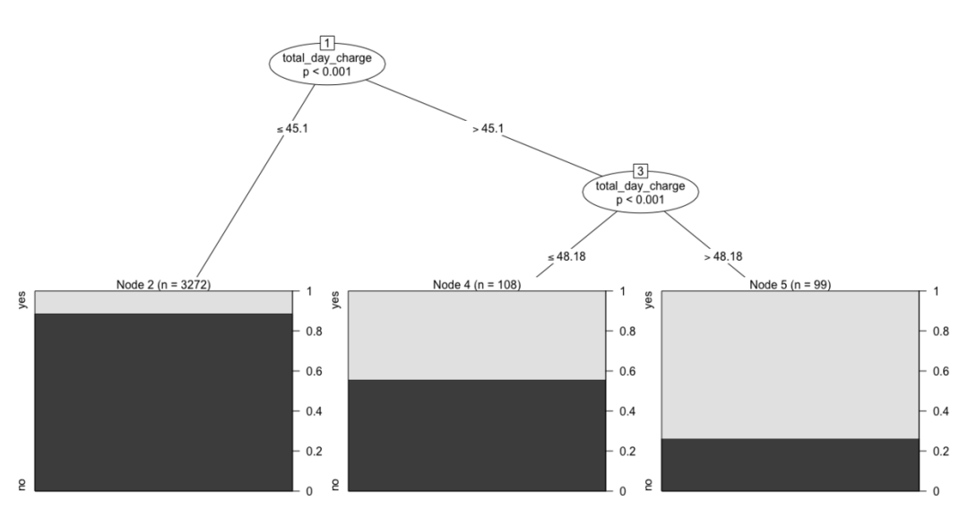
5.8 conditional reasoning tree visualization
# visualization
plot(ctree.moddel)
daycharhe.model <- ctree(churn~total_day_charge, data = trainset)
plot(daycharhe.model)

Simplify it
5.9 evaluation and prediction ability
 # forecast
> ctree.predict<- predict(ctree.moddel, testset)
> table(ctree.predict, testset$churn)

ctree.predict  yes   no
          yes  139    9
          no    75 1298
confusionMatrix(table(ctree.predict, testset$churn))
# #######################
Confusion Matrix and Statistics


ctree.predict  yes   no
          yes  139    9
          no    75 1298

               Accuracy : 0.9448
                 95% CI : (0.9321, 0.9557)
    No Information Rate : 0.8593
    P-Value [Acc > NIR] : < 2.2e-16
# probability
> treeresponse(ctree.moddel, newdata = testset[1:5,])
[[1]]
[1] 0.02715356 0.97284644

[[2]]
[1] 0.06842105 0.93157895

[[3]]
[1] 0.06842105 0.93157895

[[4]]
[1] 0.06842105 0.93157895

[[5]]
[1] 0.02715356 0.97284644
5.10 using k-adjacency classification algorithm
It is a nonparametric inert learning method, does not make any assumptions about the data distribution, and does not require the algorithm to have an explicit learning process.
install.packages("class")
library(class)
levels(trainset$international_plan) = list("0" = "no", "1" = "yes")
levels(trainset$voice_mail_plan) = list("0" = "no", "1" = "yes")
levels(testset$international_plan) = list("0" = "no", "1" = "yes")
levels(testset$voice_mail_plan) = list("0" = "no", "1" = "yes")

churn.knn <- knn(trainset[,!names(trainset) %in% c("churn", "area_code", "state" )],
                 testset[,!names(testset)  %in% c("churn", "area_code", "state" )], trainset$churn, k=3)
summary(churn.knn)
plot(churn.knn)
library(caret)
confusionMatrix(table(testset$churn,churn.knn))
# ########################
Confusion Matrix and Statistics

     churn.knn
       yes   no
  yes   76  138
  no    46 1261

               Accuracy : 0.879
                 95% CI : (0.8616, 0.895)
    No Information Rate : 0.9198
    P-Value [Acc > NIR] : 1

                  Kappa : 0.3901
knn algorithm uses similarity distance to train and classify. For example, Euclidean distance or Manhattan distance, k=1, will allocate samples to the nearest category. If K is small, it may be over fitting, too large or low fitting, and a suitable value can be obtained by cross test. The advantage is that the learning cost is 0, there is no need to assume distribution, and any type of data can be processed; The disadvantage is that it is difficult to understand, the data set is large, the calculation cost is very high, and the dimension of high-dimensional data must be reduced first. Character type data shall be processed into integer first, and k=3 shall be allocated to the last three clusters. kknn package can provide weighted k-nearest neighbor algorithm, regression and clustering.
5.11 using logistic regression
It is an algorithm based on probability and statistics. The logit function can be executed. The glm family specified as binomial is also a logical regression algorithm.
# logistic
fit <- glm(churn~., data = trainset,family = binomial)
summary(fit)
# Remove non significant variables

fit <- glm(churn~international_plan + voice_mail_plan + total_intl_calls + number_customer_service_calls , data = trainset,family = binomial)
summary(fit)
pred <- predict(fit, testset, type = "response")
pred <- predict(fit, testset, type = "response")
Class <- pred > .5
summary(Class)
   Mode   FALSE    TRUE
logical      44    1477
pred_class <- churn.mod
pred_class[pred <=.5] = 1- pred_class[pred<=.5]
ctb <- table(churn.mod, pred_class)
ctb
# ###########
         pred_class
churn.mod    0    1
        0 1287   20
        1   24  190
 confusionMatrix(ctb)
Confusion Matrix and Statistics

         pred_class
churn.mod    0    1
        0 1287   20
        1   24  190

               Accuracy : 0.9711
                 95% CI : (0.9614, 0.9789)
    No Information Rate : 0.8619
    P-Value [Acc > NIR] : <2e-16

                  Kappa : 0.8794
Logistic regression is easy to understand, directly outputs probability and confidence interval, and can quickly merge new data sets and update classification models. The disadvantage is that it cannot deal with multicollinearity, and the explanatory variables must be linear independent.
5.12 using naive Bayesian classification algorithm
It is also a probability based classifier, which assumes that the sample attributes are independent of each other.
library(e1071)
classifer <- naiveBayes(trainset[,!names(trainset) %in% c("churn")], trainset$churn)
classifer
# ##############
Naive Bayes Classifier for Discrete Predictors

Call:
naiveBayes.default(x = trainset[, !names(trainset) %in% c("churn")],
    y = trainset$churn)
# ###############
A-priori probabilities:
trainset$churn
      yes        no
0.1417074 0.8582926
bayes.table <- table(predict(classifer, testset[,!names(trainset) %in% c("churn")]), testset$churn)
bayes.table
# #############
       yes   no
  yes  104   52
  no   110 1255
library(caret)
confusionMatrix(bayes.table)
Confusion Matrix and Statistics
# ############

       yes   no
  yes  104   52
  no   110 1255

               Accuracy : 0.8935
                 95% CI : (0.8769, 0.9086)
    No Information Rate : 0.8593
    P-Value [Acc > NIR] : 4.220e-05

                  Kappa : 0.5032
Classification evaluation is based on the above routine. The naive Yess algorithm assumes that the characteristic variables are conditionally independent, with relatively simple advantages and direct application. It is suitable for training data sets with small-scale trees and possible missing or data noise. The disadvantage is that the above conditions are independent and equally important, which is difficult to achieve in the real world. To summarize this chapter, see the following pictures: