Classification of film reviews using naive Bayes

1. Data set explanation:

The data set is a subset of IMDB movie data set, which has been divided into test set and training set. The training set includes 25000 movie reviews, and there are 25000 test sets. The data set has been preprocessed to convert the specific word sequence of each review into an integer sequence in the thesaurus, in which each integer represents the position of the word in the thesaurus. For example, the integer 104 represents that the word is the 104th word of the thesaurus. For the simplicity of the experiment, the thesaurus only retained 10000 most common words, and the low-frequency words were discarded. Each comment has a tag, with 0 as a negative comment and 1 as a positive comment.

Training data in train_data.txt file, each line has a comment, and the training set label is in train_labels.txt file, each line has a comment label; Test data in test_data.txt file, the test data label is not given.

2. Concrete realization:

1. Fetch dataset:

   Take out the training set and test set from txt:

   with open("test/test_data.txt", "rb") as fr:
   
     test_data_n = [inst.decode().strip().split(' ') for inst in fr.readlines()]
   
     test_data = [[int(element) for element in line] for line in test_data_n]
   
   test_data = np.array(test_data)
   

2. Data processing:

   For each comment, first decode it into English words, then reverse the key value and map the integer index into words.

   Encode an integer sequence into a binary sequence.

   Finally, the training set label is vectorized.

   # Decode a comment into English words
   
   word_index = imdb.get_word_index() # word_index is a dictionary that maps words to integer indexes
   
   reverse_word_index = dict([(value, key) for (key, value) in word_index.items()])
   
   # The key value is reversed and the integer index is mapped to words
   
   decode_review = ' '.join(
   
     [reverse_word_index.get(i - 3, '?') for i in train_data[0]]
   
   ) 
   
   \# Decode comments
   
   \# Note that the index subtracts 3 because 0,1,2 is populated for padding
   
   \# At the beginning of the "start sequence" sequence, the indexes reserved for "unknown" unknown words
   
    
   
   \# Encoding an integer sequence into a binary matrix
   
   def vectorize_sequences(sequences, dimension=10000):
   
     results = np.zeros((len(sequences), dimension)) # Create a matrix with the shape (len(sequences), dimension)
   
     for i, sequence in enumerate(sequences):
   
       results[i, sequence] = 1 # Set the specified index of results[i] to 1
   
     return results
   
   x_train = vectorize_sequences(train_data)
   
   x_test = vectorize_sequences(test_data)
   
   \# Label Vectorization
   
   y_train = np.asarray(train_labels).astype('float32')
   

3. Modeling:

   Optional polynomial model or Bernoulli model.

   The computing granularity of the two is different. The polynomial model takes words as the granularity and the Bernoulli model takes files as the granularity. Therefore, the calculation methods of a priori probability and class conditional probability are different.
   When calculating the posterior probability, for a document d, in the polynomial model, only the words that appear in d will participate in the posterior probability calculation. In the Bernoulli model, the words that do not appear in d but appear in the global word list will also participate in the calculation, but as the "opposite side".
   When the training set document is short, that is to say, there are not many repeated words, the numerator of polynomial and Bernoulli model formula is equal, and the denominator value of polynomial is greater than Bernoulli numerator value, so the likelihood estimation value of polynomial will be less than Bernoulli's likelihood estimation value.
   Therefore, when the training set text is short, we prefer to use Bernoulli model. When the text is long, we prefer polynomial model, because the high-frequency word in a document will make the likelihood probability value of the word relatively large.

   Use Laplace smoothing

   alpha: a priori smoothing factor, which is equal to 1 by default. When equal to 1, it means Laplacian smoothing.

   # model = MultinomialNB()
   model = BernoulliNB()
   model.fit(X_train, y_train)
   

4. Output the prediction results on the test set:

   Write results to txt

   # model evaluation
   print("model accuracy is " + str(accuracy_score(y_test, y_pred)))
   print("model precision is " + str(precision_score(y_test, y_pred, average='macro')))
   print("model recall is " + str(recall_score(y_test, y_pred, average='macro')))
   print("model f1_score is " + str(f1_score(y_test, y_pred, average='macro')))
   
   des = y_pred_local.astype(int)
   np.savetxt('Text3_result.txt', des, fmt='%d', delimiter='\n')
   

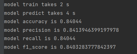
3. Experimental results:

Use polynomial model:

Nubury model:

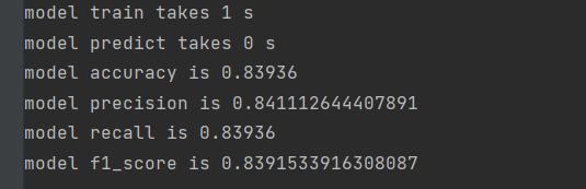
In this scenario, there is little difference between the two.

Experimental summary

1. Bayesian probability and Bayesian criterion provide an effective method to estimate location probability by using known values;
2. Naive Bayes assumes that the data features are independent of each other. Although this assumption is not strictly true in general, using naive Bayes for classification can still achieve good results;
3. Advantages of Bayesian network: it is still effective in the case of less data, and can deal with multi category problems;
4. The disadvantage of Bayesian network: it is sensitive to the preparation of input data.
5. Laplace smoothing plays a positive role in improving the classification effect of naive Bayesian classifier.