Measuring the performance of clustering algorithm is not simply counting the number of errors or calculating the precision and recall in supervised classification algorithm. There are many evaluation indicators for clustering algorithms. This paper is mainly based on the sklearn machine learning library, which provides a series of measurement functions. In these measurement functions, some need to know the real sample categories, and then some clustering have no real sample categories, and even the clustering methods such as DBSCAN are uncertain about how many categories there are, How to evaluate the quality of clustering? This paper focuses on "clustering evaluation without real labels".

1, Clustering evaluation index in sklearn

1.1 introduction to clustering

Clustering is an unsupervised learning algorithm. The label of the training sample is unknown. According to the internal properties and laws of a certain standard or data, the sample is divided into several disjoint subsets. Each subset is called a cluster. Each cluster contains at least one object, and each object belongs to and only belongs to one cluster; The data similarity within clusters is high, and the data similarity between clusters is very low. Clustering can be used as a precursor process for other learning tasks such as classification.

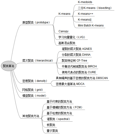
Based on different learning strategies, clustering algorithms can be divided into many types:

1.2 complete collection of sklearn clustering evaluation functions

There are many clustering evaluation indicators in sklearn, as shown below

 

   

    

   
   

    

     metrics.adjusted_mutual_info_score(...[, ...])	
    
   

   

    

   
   

    

     metrics.adjusted_rand_score(labels_true, ...)	
    
   

   

    

   
   

    

     metrics.calinski_harabasz_score(X, labels)	
    
   

   

    

   
   

    

     metrics.davies_bouldin_score(X, labels)
    
   

   

    

   
   

    

     metrics.completeness_score(labels_true, ...)	
    
   

   

    

   
   

    

     metrics.cluster.contingency_matrix(...[, ...])	
    
   

   

    

   
   

    

     metrics.fowlkes_mallows_score(labels_true, ...)	
    
   

   

    

   
   

    

     metrics.homogeneity_completeness_v_measure(...)	
    
   

   

    

   
   

    

     metrics.homogeneity_score(labels_true, ...)	
    
   

   

    

   
   

    

     metrics.mutual_info_score(labels_true, ...)	
    
   

   

    

   
   

    

     metrics.normalized_mutual_info_score(...[, ...])	
    
   

   

    

   
   

    

     metrics.silhouette_score(X, labels[, ...])	
    
   

   

    

   
   

    

     metrics.silhouette_samples(X, labels[, metric])
    
   

   

    

   
   

    

     metrics.v_measure_score(labels_true, labels_pred)	
    
   
 

Some of these evaluation functions need "parameter label_true", but there are many times when clustering does not have a real category, so this paper does not consider this type first, but only considers that label is not required_ Three evaluation functions of true.

External metrics: metrics that need to know the real label

Internal measurement: when the real clustering label does not know

2, Three evaluation functions (no label_true)

2.1} contour coefficient

Contour coefficient is an evaluation method of clustering effect. It was first proposed by Peter J. rousseuw in 1986. It combines cohesion and separation. It can be used to evaluate the impact of different algorithms or different operation modes of algorithms on the clustering results on the basis of the same original data.

Specific methods:

(1) Calculate the average distance ai from sample i to other samples in the same cluster. The smaller the ai, the more sample i should be clustered into this cluster. ai is called the intra cluster dissimilarity of sample i. The a i mean of all samples in a cluster C is called the cluster dissimilarity of cluster C.

(2) Calculate the average distance bij of all samples from sample i to other cluster Cj, which is called the dissimilarity between sample i and cluster Cj. It is defined as the dissimilarity between clusters of sample i: Bi = min {BI1, Bi2,..., bik}, that is, the dissimilarity between clusters of a sample is the smallest of the average distance between the sample and all samples of all other clusters.

The larger the bi, the less the sample i belongs to other clusters.

(3) According to the intra cluster dissimilarity a i and inter cluster dissimilarity b i of sample i, the contour coefficient of a sample i is defined:

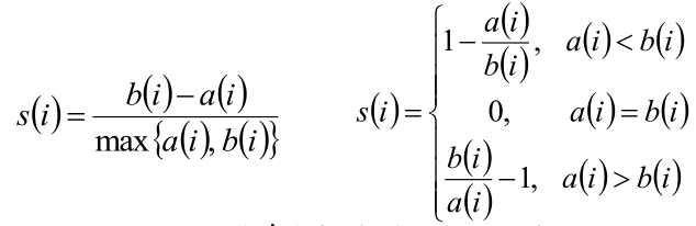
(4) Judgment:

If si is close to 1, sample i clustering is reasonable;

If si is close to - 1, sample i should be classified into another cluster;

If si is approximately 0, it means that sample i is on the boundary of two clusters.

(5) Contour coefficient S for all samples

The mean of s i of all samples is called the contour coefficient of clustering results, defined as s, which is a measure of whether the clustering is reasonable and effective. The value of the contour coefficient of the clustering results is between [- 1,1]. The larger the value, the closer the same samples are, and the farther the different samples are, the better the clustering effect is.

Summary of advantages and disadvantages of contour coefficient:

advantage

• For incorrect clustering, the score is - 1 and high density clustering is + 1. Scores near the zero point represent overlapping clusters.
• When clusters are dense and well separated, the score is higher, which is related to the standard concept of cluster.

shortcoming

• The silver coefficient of convex clusters is usually higher than other types of clusters, such as density based clusters obtained through DBSCAN.

Interface in sklearn:

Contour coefficient and other evaluation functions are defined in sklearn In the metrics module,

Function silhouette in sklearn_ Score() calculates the average contour coefficient of all points, while silhouette_samples() returns the contour coefficient for each point. Specific examples will be given later. It is defined as follows:

 

   

    

   
   

    

     def 
     silhouette_score(
     X, labels, metric='euclidean', sample_size=None,
    
   

   

    

   
   

    

     random_state=None, **kwds):
    
   

   

    

   
   

    

     '''
    
   

   

    

   
   

    

     X: Represents the sample data to be clustered, generally in the form of( samples，features)Format of
    
   

   

    

   
   

    

     labels: That is, after clustering label Label, shaped as( samples，)Format of
    
   

   

    

   
   

    

     metric: The default is Euclidean distance
    
   

   

    

   
   

    

     '''
    
   
 

2.2 CH score (Calinski Harabasz Score)

Also known as calinski harabaz index

This calculation is simple and direct. The larger the calinski harabasz score ss, the better the clustering effect. The mathematical calculation formula of calinski harabasz score value ss is (theoretical introduction comes from: learning K-Means clustering with scikit learn):

Namely

among

Bk is called between clusters dispersion mean

Wk calls it within cluster dispersion

Their calculation formula is as follows:

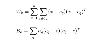
The smaller the covariance of the data within the category, the better, and the larger the covariance between the categories, the better. In this way, the calinski harabasz score will be higher. To sum up:

The higher the value of CH index, the better.

When the real clustering label is unknown, it can be used as an indicator of the evaluation model. At the same time, the smaller the value, it can be understood that the covariance between groups is very small, and the boundary between groups is not obvious. Compared with the contour coefficient, the author thinks the biggest advantage: fast! Hundreds of times! In milliseconds,

Summary of advantages and disadvantages:

advantage

• When clusters are dense and well separated, the score is higher, which is related to a standard cluster.
• Score calculation is fast

shortcoming

• The calinski harabaz index of convex clusters is usually higher than other types of clusters, such as density based clusters obtained through DBSCAN.

Interface in sklearn:

In scikit learn, the method corresponding to calinski harabasz index is metrics calinski_ harabaz_ score. It is defined as follows:

 

   

    

   
   

    

     def 
     calinski_harabasz_score(
     X, labels):
    
   

   

    

   
   

    

     '''
    
   

   

    

   
   

    

     X: Represents the sample data to be clustered, generally in the form of( samples，features)Format of
    
   

   

    

   
   

    

     labels: That is, after clustering label Label, shaped as( samples，)Format of
    
   

   

    

   
   

    

     '''
    
   
 

2.3 # Davidson boding index (DBI) - davies_bouldin_score

Davidson bauding index (DBI), also known as classification accuracy index, is an index proposed by David L. Davis and Donald Bouldin to evaluate the advantages and disadvantages of clustering algorithm. Firstly, suppose we have m time series, which are clustered into n clusters. M time series are set as input matrix X, and N cluster classes are set as n as parameters. Calculate using the following formula:

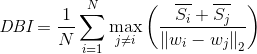
The meaning of this formula is to measure the mean value of the maximum similarity of each cluster class.

Next is the specific calculation steps of the algorithm:

(1) Calculate Si. DBI defines a dispersion value Si: it represents the dispersion degree of measured data points in the ith class,

The Si variable is first defined in the DBI calculation formula. Si calculates the average distance from the data in the class to the cluster centroid, representing the dispersion degree of each sample in cluster i. The calculation formula is:

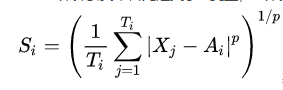
Where Xj represents the j-th data point in cluster i, that is, a sample point, Ai is the centroid of cluster i, Ti is the number of data in cluster i, and p is usually taken as 2, so that the euclidean metric between the independent data point and the centroid can be calculated. At this time, it represents the standard deviation of the distance from each point to the center, They can be used to measure the degree of dispersion. Of course, Euclidean distance may not be the best distance calculation method when investigating flow patterns and high-dimensional data, but it is also typical.

(2) Calculate Mij. DBI defines a distance value Mij: represents the distance between class i and class j,

After the sum of molecules is calculated, the denominator Mij needs to be calculated, which is defined as the distance between cluster i and cluster j, and the calculation formula is:

ak,i represents the k-th value of the centroid of cluster i, and Mij is the distance between the centroid of cluster i and cluster j. That is, aki represents the value of the k-th attribute of the center point of class i, and Mij is the distance between the center of class i and the center of class j.

(3) Calculate Rij. DBI defines a similarity value Rij:
Rij measures the similarity between class i and class j. The calculation formula is:

(4) Calculate DBI

Through the calculation of the above formula, we select the maximum value Ri=max (Rij) from Rij, that is, the value of the maximum similarity between class i and other classes.

Finally, calculate the mean of these maximum similarity of each class to obtain the DBI index:

The smaller the value, the better the classification effect.

Note: the minimum value of DBI is 0. The smaller the value, the better the clustering effect.

Definitions in DBI's sklearn:

 

   

    

   
   

    

     def 
     davies_bouldin_score(
     X, labels):
    
   

   

    

   
   

    

     '''
    
   

   

    

   
   

    

     X: Represents the sample data to be clustered, generally in the form of( samples，features)Format of
    
   

   

    

   
   

    

     labels: That is, after clustering label Label, shaped as( samples，)Format of
    
   

   

    

   
   

    

     '''
    
   
 

3, Actual case

The actual case will show the usage of these three evaluation indicators. The clustering algorithm used is DBSCAN algorithm,

3.1 the original samples are as follows:

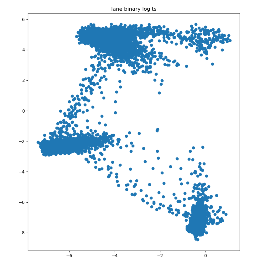
The data dimension is (7283,2), that is, each point is a two-dimensional vector. As for how this data comes from, it is actually my own data in the project. I can generate or find some other data myself.

3.2 clustering using DBSCAN

The results after clustering are:

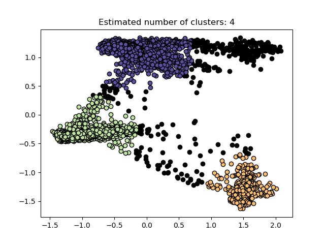
It can be seen that it is divided into three categories. Black represents noise points. The principle of DBSCAN clustering will not be expanded here,

3.3 evaluation function

Here you can refer to the complete code

 

   

    

   
   

    

     import numpy 
     as np
    
   

   

    

   
   

    

     import matplotlib.pyplot 
     as plt
    
   

   

    

   
   

    

     import glog 
     as log
    
   

   

    

   
   

    
 
    
   

   

    

   
   

    

     from sklearn.cluster 
     import DBSCAN  
     # DBSCAN clustering
    
   

   

    

   
   

    

     from sklearn.preprocessing 
     import StandardScaler
    
   

   

    

   
   

    

     from sklearn.metrics 
     import silhouette_score ,calinski_harabasz_score,davies_bouldin_score 
     # Calculate contour coefficient, CH index, DBI 
    
   

   

    

   
   

    
 
    
   

   

    

   
   

    
 
    
   

   

    

   
   

    

     # Define a function for DBSCAN
    
   

   

    

   
   

    

     def 
     DBSCAN_Cluster(
     embedding_image_feats):
    
   

   

    

   
   

    
    
     """
    
   

   

    

   
   

    

         dbscan cluster
    
   

   

    

   
   

    

         :param embedding_image_feats:  # For example, the shape (9434,4) represents 9434 pixels
    
   

   

    

   
   

    

         :return:
    
   

   

    

   
   

    

         """
    
   

   

    

   
   

    

         db = DBSCAN(eps=
     0.35, min_samples=
     600)
    
   

   

    

   
   

    
    
     try:
    
   

   

    

   
   

    

             features = StandardScaler().fit_transform(embedding_image_feats)  
     # Normalize features
    
   

   

    

   
   

    

             db.fit(features)
    
   

   

    

   
   

    
    
     except Exception 
     as err:
    
   

   

    

   
   

    

             log.error(err)   
    
   

   

    

   
   

    

             ret = {
    
   

   

    

   
   

    
            
     'origin_features': 
     None,
    
   

   

    

   
   

    
            
     'cluster_nums': 
     0,
    
   

   

    

   
   

    
            
     'db_labels': 
     None,
    
   

   

    

   
   

    
            
     'cluster_center': 
     None
    
   

   

    

   
   

    

                 }
    
   

   

    

   
   

    
        
     return ret
    
   

   

    

   
   

    
 
    
   

   

    

   
   

    

         db_labels = db.labels_                  
     # After obtaining the cluster, there is no category label of a sample
    
   

   

    

   
   

    

         unique_labels = np.unique(db_labels)    
     # Get a unique category
    
   

   

    

   
   

    
 
    
   

   

    

   
   

    

         num_clusters = 
     len(unique_labels)
    
   

   

    

   
   

    

         cluster_centers = db.components_
    
   

   

    

   
   

    
 
    
   

   

    

   
   

    

         ret = {
    
   

   

    

   
   

    
            
     'origin_features': features,      
     #(9434,4)
    
   

   

    

   
   

    
            
     'cluster_nums': num_clusters,     
     # 5 it is a scalar, representing 5 classes, including the background
    
   

   

    

   
   

    
            
     'db_labels': db_labels,           
     #(9434,)
    
   

   

    

   
   

    
            
     'unique_labels': unique_labels,   
     #(5,)
    
   

   

    

   
   

    
            
     'cluster_center': cluster_centers 
     #(6425,4)
    
   

   

    

   
   

    

             }
    
   

   

    

   
   

    
 
    
   

   

    

   
   

    
    
     return ret
    
   

   

    

   
   

    
 
    
   

   

    

   
   

    

     # Draw the results after clustering
    
   

   

    

   
   

    

     def 
     plot_dbscan_result(
     features,db_labels,unique_labels,num_clusters):
    
   

   

    

   
   

    

         colors = plt.cm.Spectral(np.linspace(
     0, 
     1, 
     len(unique_labels)))
    
   

   

    

   
   

    
    
     for k, color 
     in 
     zip(unique_labels, colors):
    
   

   

    

   
   

    
        
     if k == -
     1:
    
   

   

    

   
   

    

                color = 
     'k'  
     # Black, which represents the noise point
    
   

   

    

   
   

    
 
    
   

   

    

   
   

    

             index=np.where(db_labels==k)   
     #  Get the index position of each category
    
   

   

    

   
   

    

             x=features[index]
    
   

   

    

   
   

    
 
    
   

   

    

   
   

    

             plt.plot(x[:, 
     0], x[:, 
     1], 
     'o', markerfacecolor=color,markeredgecolor=
     'k', markersize=
     6)
    
   

   

    

   
   

    
 
    
   

   

    

   
   

    

         plt.title(
     'Estimated number of clusters: %d' % num_clusters)
    
   

   

    

   
   

    

         plt.show()
    
   

   

    

   
   

    
 
    
   

   

    

   
   

    
 
    
   

   

    

   
   

    

     if __name__==
     '__main__':
    
   

   

    

   
   

    

         embedding_features=np.load(
     "./tools/features_logits/lane_embedding_feats.npy")  
     # Import data in the format of (samples,)
    
   

   

    

   
   

    
 
    
   

   

    

   
   

    

         ret=DBSCAN_Cluster(embedding_features)  
     # DBSCAN clustering
    
   

   

    

   
   

    
 
    
   

   

    

   
   

    

         plot_dbscan_result(ret[
     'origin_features'],ret[
     'db_labels'],ret[
     'unique_labels'],ret[
     'cluster_nums']) 
     # Show the results after clustering
    
   

   

    

   
   

    
 
    
   

   

    

   
   

    
    
    
   

   

    

   
   

    

         s1=silhouette_score(embedding_features, ret[
     'db_labels'], metric=
     'euclidean') 
     # Calculate contour coefficient
    
   

   

    

   
   

    

         s2=calinski_harabasz_score(embedding_features,ret[
     'db_labels']) 
     # Calculate CH score
    
   

   

    

   
   

    

         s3=davies_bouldin_score(embedding_features,ret[
     'db_labels'])    
     # Calculate DBI
    
   

   

    

   
   

    
 
    
   

   

    

   
   

    
    
     print(s1)
    
   

   

    

   
   

    
    
     print(s2)
    
   

   

    

   
   

    
    
     print(s3)
    
   

   

    

   
   

    
 
    
   

   

    

   
   

    

     '''The operation result is:
    
   

   

    

   
   

    

     0.7971864
    
   

   

    

   
   

    

     48375.80213812995
    
   

   

    

   
   

    

     0.8799878743935938
    
   

   

    

   
   

    

     '''