Common probability density images in Statistics

Reviewing probability theory and mathematical statistics today, I saw several common distributions and suddenly became interested, so I tried to write about them matlab Draw several common probability density images (Note: some are collected and sorted from the Internet)

Binomial:

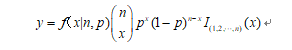
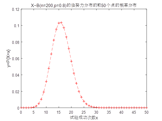
Binomial distribution, also known as n-fold Bernoulli effort test, the success probability of each experiment is p, and the failure probability is q=1-p, then in this n independent experiments, the probability of success x times is y

clc;
clear;
x= 0:50;
y = binopdf(x,200,0.08);%Binomial probability density function
plot(x,y,'--r+');%Mapping
title('X~B(n=200,p=0.8)The probability distribution of the first 50 points of the Bernoulli distribution');
xlabel('Number of successful tests x');%x label
ylabel('y=P\{X=x\}');%y label

distribution

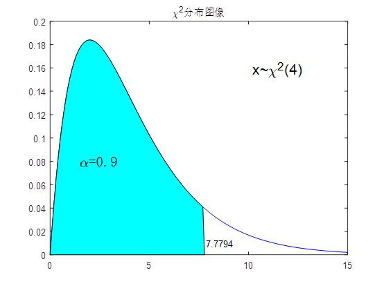
If n independent random variables ξ ₁， ξ ₂，..., ξ n. All comply with the standard Normal distribution (also known as independent and identically distributed in the standard normal distribution), then the sum of the squares of these n random variables subject to the standard normal distribution constitutes a new random variable, and its distribution law is called chi square distribution.

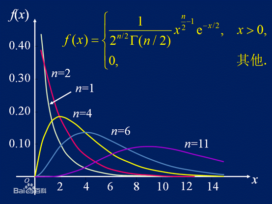
n=4;%Chi square distribution parameters: freedom
P=0.9;%P value
x_xi=chi2inv(P,n); % according to P Value inverse check critical value
%----Draw chi square distribution map--------------
x=0:0.1:15;
yd_c=chi2pdf(x,n); %Obtain the corresponding density distribution value
plot(x,yd_c,'b'),hold on %Draw a picture
 
%Draw the shaded portion of the distribution function-------------
xxf=0:0.1:x_xi;% 0~critical value
yyf=chi2pdf(xxf,n); 
fill([xxf,x_xi],[yyf,0],'c') %Fill with blue
%Add dimension
text(x_xi*1.01,0.01,num2str(x_xi)) %Dimension critical value
text(10,0.16,['\fontsize{16} x~{\chi}^2' '(4)'])    %Label distribution name
text(1.5,0.08,'\fontname{official script}\fontsize{16}\alpha=0.9') %tagging P value
title('\chi^2 Distribution image')
hold off 
 

Normal distribution

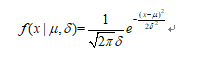
Normal distribution, also known as "normal distribution", also known as Gaussian distribution, was first obtained by A. dimofer in the asymptotic formula of binomial distribution. C.F. Gauss derived it from another angle when studying the measurement error. P.S. Laplace and Gauss studied its properties. It is a very important probability distribution in the fields of mathematics, physics and engineering. It has a great influence in many aspects of statistics. The normal curve is bell shaped, with low ends, high middle and symmetrical left and right. Because its curve is bell shaped, it is often called bell shaped curve. If the random variable X obeys a mathematical expectation μ, Variance is σ^ The normal distribution of 2 is recorded as n( μ，σ^ 2). The probability density function is the expected value of normal distribution μ Determines its position and its standard deviation σ Determines the magnitude of the distribution. When μ = 0 σ = The normal distribution at 1 is the standard normal distribution.

clc;
clear;
mu=3;
sigma=0.5;
x=mu+sigma*[-3:-1,1:3];
yf=normcdf(x,mu,sigma); 
P=[yf(4)-yf(3),yf(5)-yf(2),yf(6)-yf(1)];
xd=1:0.1:5;
yd=normpdf(xd,mu,sigma); % 
for k=1:3 
    xx{k}=x(4-k):sigma/10:x(3+k);
    yy{k}=normpdf(xx{k},mu,sigma);
end
subplot(1,3,1),plot(xd,yd,'r');
hold on 
fill([x(3),xx{1},x(4)],[0,yy{1},0],'c') 
text(mu-0.5*sigma,0.3,num2str(P(1))),hold off
subplot(1,3,2),plot(xd,yd,'r');
hold on 
fill([x(2),xx{2},x(5)],[0,yy{2},0],'c') 
text(mu-0.5*sigma,0.3,num2str(P(2))),hold off
subplot(1,3,3),plot(xd,yd,'r');
hold on
fill([x(1),xx{3},x(6)],[0,yy{3},0],'c')
text(mu-0.5*sigma,0.3,num2str(P(3))),hold off   

clc,clear
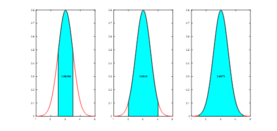
mu=2.5;sigma=0.6;
x=(mu-4*sigma):0.005:(mu+4*sigma);
y=normcdf(x,mu,sigma);
f=normpdf(x,mu,sigma);
[M,V]=normstat(mu,sigma)
plot(x,y,'-r',x,f,'-b')
legend('pdf','cdf')
grid  on

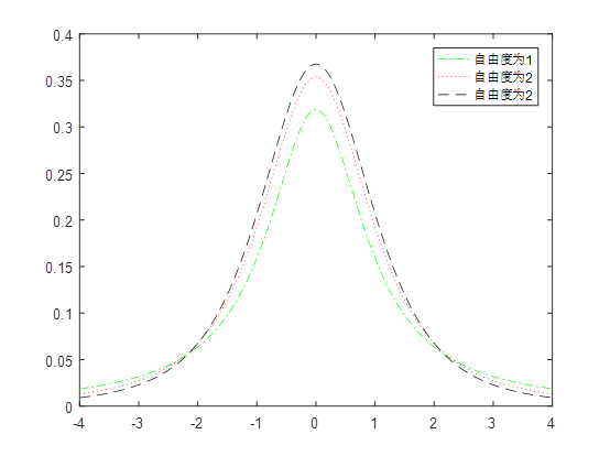
T distribution

In probability theory and statistics, student t-distribution, which can be abbreviated as t-distribution, is used to estimate the mean value of the population with normal distribution and unknown variance according to small samples. If the population variance is known (for example, when the number of samples is large enough), the normal distribution should be used to estimate the population mean. The shape of t distribution curve is related to the size of n (specifically, the degree of freedom df). Compared with the standard normal distribution curve, the smaller the degree of freedom df is, the flatterer the t distribution curve is, the lower the middle of the curve is, and the higher the tail of both sides of the curve is; The greater the degree of freedom df, the closer the t-distribution curve is to the normal distribution curve. When the degree of freedom df = ∞, the t-distribution curve is the standard normal distribution curve.

clc
clear
x=-4:0.01:4;
%t Distribution probability density function
y=tpdf(x,1)
y1=tpdf(x,2)
y2=tpdf(x,3)
plot(x,y,'-.',x,y1,':',x,y2,'--')%Mapping
axis([-4,4,0,0.4])%Limit coordinates
legend('The degree of freedom is 1','The degree of freedom is 2','The degree of freedom is 2')%Add label

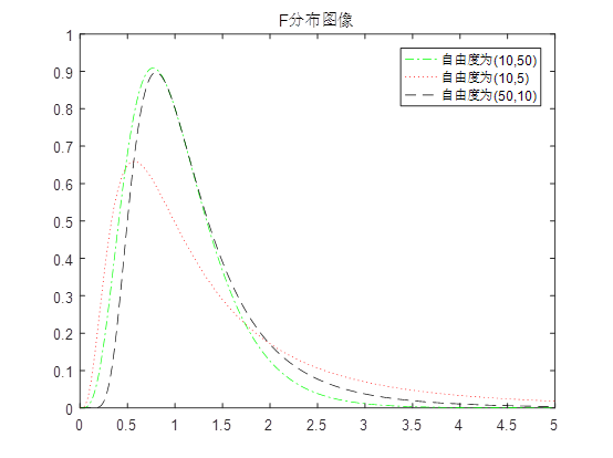
F distribution

The F distribution was proposed by the British statistician R.A.Fisher in 1924 and named after the first letter of his surname. It is an asymmetric distribution with two degrees of freedom and its position is not interchangeable. F distribution has a wide range of applications, such as analysis of variance and significance test of regression equation.

clc
clear
x=0:0.01:5;
%t Distribution probability density function
y=fpdf(x,10,50)
y1=fpdf(x,10,5)
y2=fpdf(x,50,10)
plot(x,y,'g-.',x,y1,'r:',x,y2,'k--')%Mapping
legend('The degree of freedom is(10,50)','The degree of freedom is(10,5)','The degree of freedom is(50,10)')%Add label
title('F Distribution image')

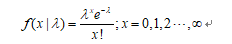
Poisson distribution

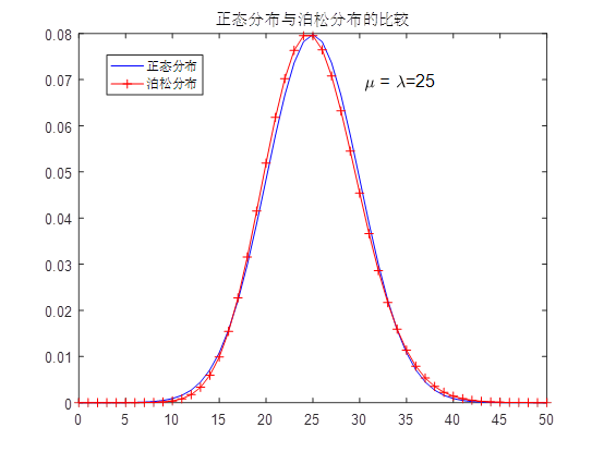
Parameters of Poisson distribution λ Is the average incidence of random events per unit time (or unit area). Poisson distribution is suitable to describe the number of random events in unit time.

clc;
clear;
Lambda=25;
x=0:50;
p=poisspdf(x,Lambda);%Poisson distribution probability distribution function
y=normpdf(x,Lambda,sqrt(Lambda));%Normal distribution probability distribution function
plot(x,y,'b-',x,p,'r-+')%Mapping
title('Comparison between normal distribution and Poisson distribution')
legend('Normal distribution','Poisson distribution ')
text(30,0.07,'\fontsize{12} {\mu} = {\lambda}=25')