Write before:

Hello, I'm time.

What we bring today is the quick sort in the sorting algorithm.
I explained it graphically and tried to write it thoroughly. Don't say much, let's go!

Mind map:

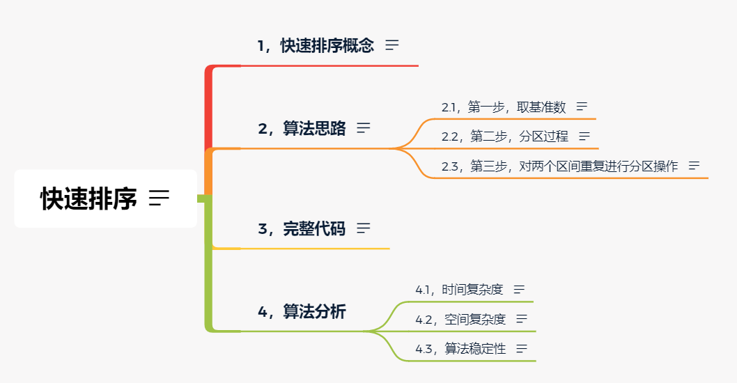
1. Quick sort concept

The records to be arranged are separated into two independent parts by one-time sorting. If the keywords of one part of the records are smaller than those of the other part, the records of the two parts can be sorted separately to achieve the order of the whole sequence. The divide and conquer method and the number of excavation and filling are mainly adopted. The divide and conquer method is to decompose the big problem into small problems and pile up small problems to solve, so that the big problem can be solved.

2. Algorithm idea

Let's make clear the idea of heap sorting first, and make clear the logic first, so as not to rush to write code.

We first have an unordered array, for example

int[] arr={4,2,8,0,5,7,1,3,9};

2.1. Step 1: take the benchmark number

Reference number (pivot): take the first element of the array. At this time, the reference number: arr[0]=4

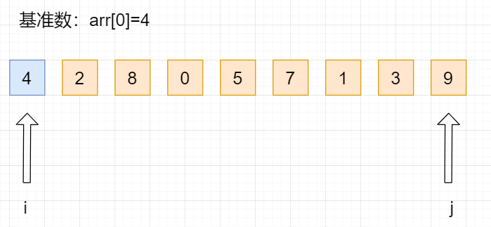
Two variables i and j are defined to point to the first element start and the last element end of the unordered array, respectively.

//start
int i=start;
int j=end;
//Get base number
int temp=arr[start];

2.2, step 2, partition process

In the partition process, all numbers larger than the benchmark number are placed on its right, and all numbers smaller or equal than the benchmark number are placed on its left.

First, we define the first element arr[0]=4 as the reference element. At this time, the first position of the array is the pit. Then we should start from the right to the left of the array to find the elements less than the reference number and exchange positions with the pit.

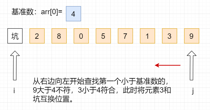
while(i<j){
    //From right to left, find the one smaller than the benchmark number
    while(i<j&&arr[j]>=temp){
        j--;
    }
    //Judge the equality and fill the pit
    if(i<j){
        arr[i]=arr[j];
        i++;
    }
}

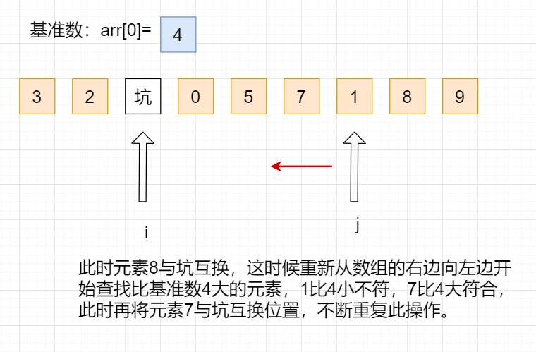
After changing the position, now convert to find elements larger than the benchmark number from the left to the right of the array:

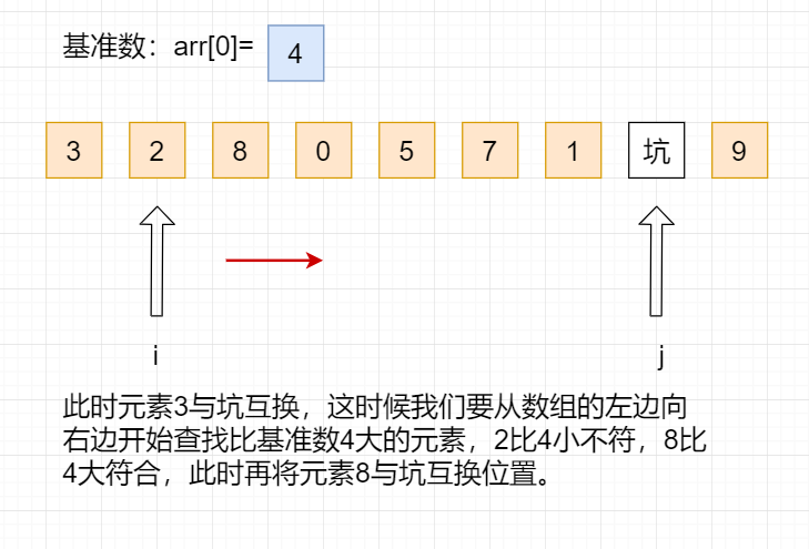
while(i<j){
    //From right to left, find the one smaller than the benchmark number
    while(i<j&&arr[j]>=temp){
        j--;
    }
    //Judge the equality and fill the pit
    if(i<j){
        arr[i]=arr[j];
        i++;
    }
    //Look from left to right for a larger number than the benchmark
    while(i<j&&arr[i]<temp){
        i++;
    }
    //Judge the equality and fill the pit
    if(i<j){
        arr[j]=arr[i];
        j--;
    }
}

After changing the position, now start looking for elements smaller than the benchmark number from the right to the left of the array again:

Repeat this operation until it is divided into left and right partitions, and then fill the benchmark number into the pit, so that the first sequence is completed. As follows:

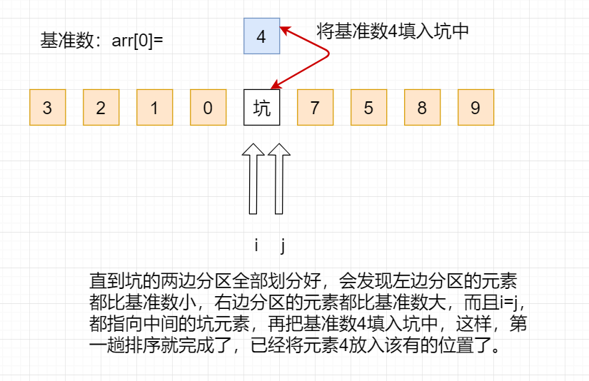
//Put the reference number at i=j
arr[i]=temp;

2.3. Step 3: repeat the partition operation for the two sections

Here, we repeat the above partition operation for the divided two intervals until there is only one element in each interval.

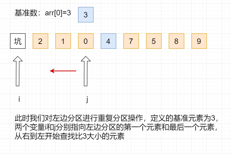
Repeat the above operations until the left and right partitions are arranged in order, and the whole sorting process is completed:

//Quickly arrange the left half
QuickSort(arr,start,i-1);
//Quickly arrange the right half
QuickSort(arr,i+1,end);

3. Complete code

import java.util.Arrays;

public class Quick_Sort {
    public static void main(String[] args) {
        int[] arr=new int[]{4,2,8,0,5,7,1,3,9};
        System.out.println(Arrays.toString(QuickSort(arr,0,arr.length-1)));
    }

    public static int[] QuickSort(int[] arr,int start,int end){
        //start
        int i=start;
        int j=end;
        //Get base number
        int temp=arr[start];
        //I < J is the cycle condition
        if(i<j){
            while(i<j){
                //From right to left, find the one smaller than the benchmark number
                while(i<j&&arr[j]>=temp){
                    j--;
                }
                //Judge the equality and fill the pit
                if(i<j){
                    arr[i]=arr[j];
                    i++;
                }
                //Look from left to right for a larger number than the benchmark
                while(i<j&&arr[i]<temp){
                    i++;
                }
                //Judge the equality and fill the pit
                if(i<j){
                    arr[j]=arr[i];
                    j--;
                }
            }
            //Put the reference number at i=j
            arr[i]=temp;
            //Quickly arrange the left half
            QuickSort(arr,start,i-1);
            //Quickly arrange the right half
            QuickSort(arr,i+1,end);
        }
        return arr;
    }
}

4. Algorithm analysis

4.1 time complexity

The worst time complexity of quick sort is O(n^2), and the best time complexity is O(nlogn), so the average time complexity is finally calculated as O(nlogn).

4.2 spatial complexity

The spatial complexity is O(1) because no additional set space is used.

4.3, algorithm stability

Quick sorting is an unstable sorting algorithm. Because we cannot guarantee that equal data is scanned and stored in order.

The worst time complexity is O(n^2), and the best time complexity is O(nlogn), so the average time complexity is finally calculated as O(nlogn).

4.2 spatial complexity

The spatial complexity is O(1) because no additional set space is used.

4.3, algorithm stability

Quick sorting is an unstable sorting algorithm. Because we cannot guarantee that equal data is scanned and stored in order.