Convolutional neural network of pytorch task05

Article directory

Convolutional neural network of pytorch task05

1. Basis of convolution neural network

1.1 two dimensional convolution
1.2 filling and stride
1.3 multiple input channels and multiple output channels
1.4 comparison between convolution layer and full connection layer
1.5 pools

2. Classic model

LeNet-5
AlexNet
VGG
GoogLeNet (Inception)
ResNet

Degradation problem
The solution of residual network

3. Construction of convolution neural network model

Convolutional Neural Network

1. Basis of convolution neural network

1.1 two dimensional convolution

The input of two-dimensional cross correlation operation is a two-dimensional input array and a two-dimensional kernel array, and the output is also a two-dimensional array, in which the kernel array is usually called convolution kernel or filter. The size of the convolution kernel is usually smaller than the input array. The convolution kernel slides on the input array. At each position, the convolution kernel multiplies and sums the input subarray at that position by elements to get the elements of the corresponding position in the output array. Figure 1 shows an example of cross-correlation operation. The shadow part is the first calculation area of input, core array and corresponding output.

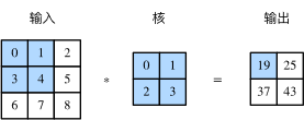
Fig. 1 two dimensional cross correlation operation

*Characteristic map and receptive field*

The two-dimensional array output from the two-dimensional convolution layer can be regarded as a representation of the input at a certain level in the spatial dimension (width and height), also known as feature map. All possible input areas that affect the forward calculation of element xx (which may be larger than the actual size of the input) are called receptive field s of xx.

Taking Figure 1 as an example, the four elements in the shadow part of the input are the receptive fields of the elements in the shadow part of the output. The output with the shape of 2 × 22 × 2 in the graph is recorded as YY, and the cross-correlation operation between YY and another core array with the shape of 2 × 22 × 2 is performed to output a single element zz. So, zz's receptive field on YY includes all four elements of YY, and its receptive field on input includes all nine elements. It can be seen that a deeper convolution neural network can make the receptive field of single element in the feature map wider, so as to capture the features with larger size on the input.

1.2 filling and stride

*padding refers to filling elements (usually 0 elements) on both sides of the input height and width. In Figure 2, elements with values of 0 are added on both sides of the original input height and width respectively.

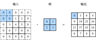
Fig. 2 two dimensional cross correlation calculation with 0 element filled on both sides of the input height and width

If the height and width of the original input are nhnh and nwnw, the height and width of the convolution kernel are khkh and kwkw, phph lines are filled on both sides of the height and pwpw columns are filled on both sides of the width, the output shape is:

(nh+ph−kh+1)×(nw+pw−kw+1)(nh+ph−kh+1)×(nw+pw−kw+1)

In the cross-correlation operation, the convolution kernel slides on the input array, and the number of rows and columns per slide is * stride *. The previous steps are all 1, and figure 3 shows the two-dimensional cross-correlation operation of step 3 in height and step 2 in width.

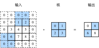
Fig. 3 two dimensional cross-correlation operation with height and width steps of 3 and 2 respectively

Generally speaking, when the high step is shsh and the wide step is swsw, the output shape is:

⌊(nh+ph−kh+sh)/sh⌋×⌊(nw+pw−kw+sw)/sw⌋ \lfloor(n_h+p_h-k_h+s_h)/s_h\rfloor \times \lfloor(n_w+p_w-k_w+s_w)/s_w\rfloor ⌊(nh+ph−kh+sh)/sh⌋×⌊(nw+pw−kw+sw)/sw⌋

If ph=kh − 1ph=kh − 1, pw=kw − 1pw=kw − 1, the output shape will be simplified to ⌊ (nh+sh − 1)/sh ⌋ ×⌊ (nw+sw − 1)/sw ⌋ (nh+sh − 1)/sh ⌋ (nw+sw − 1)/sw ⌋. Further, if the input height and width can be divided by the strides on the height and width respectively, the output shape will be (nh/sh) × (nw/sw)(nh/sh) × (nw/sw).

When ph=pw=pph=pw=p, the filling is called pp; when sh=sw=ssh=sw=s, the stride is called ss.

In the convolution neural network, we use the odd high and wide kernel, such as 3 × 33 × 3, 5 × 55 × 5 convolution kernel. For the kernel whose height (or width) is 2k+12k+1, and whose stride is 1, we can keep the same size of input and output by selecting the filling whose size is kk on both sides of the height (or width).

1.3 multiple input channels and multiple output channels

Multiple input channels

The input of convolution layer can contain multiple channels, and Figure 4 shows an example of two-dimensional cross-correlation calculation with two input channels.

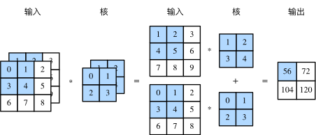
Figure 4 cross correlation calculation with two input channels

Assuming that the number of channels of input data is cici and the shape of convolution kernel is kh × kwkh × kw, each input channel is assigned a kernel array with the shape of kh × kwkh × kw. The two-dimensional output of the cross-correlation operation of cici is added by channels, and a two-dimensional array is obtained as the output. A convolution kernel with the shape of ci × kh × kwci × kh × kw is obtained by connecting the array of cici cores on the channel dimension.

Multiple output channels

The output of convolution layer can also contain multiple channels. The number of input channels and output channels of convolution kernel are cici and coco respectively, and the height and width are khkh and kwkw respectively. If you want to get the output with multiple channels, you can create a core array with the shape of ci × kh × kwci × kh × kw for each output channel, and connect them in the output channel dimension. The convolution core shape is co × ci × kh × kwco × ci × kh × kw.

For the convolution kernel of output channel, this paper provides an understanding that a core array of ci × kh × kwci × kh × kw can extract some local features, but the input may have quite rich features, which requires multiple core arrays of ci × kh × kwci × kh × kw. Different core groups extract different features.

1x1 volume layer

Finally, the convolution kernel with the shape of 1 × 11 × 1 is discussed. Generally, the convolution operation is called 1 × 11 × 1 convolution. The convolution layer including the convolution kernel is called 1 × 11 × 1 convolution layer. Figure 5 shows the cross correlation calculation using a 1 × 11 × 1 convolution kernel with 3 input channels and 2 output channels.

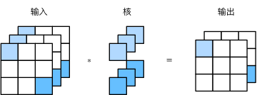
Fig. 5 cross correlation calculation of 1x1 convolution kernel. Input and output have the same height and width

The 1 × 11 × 1 convolution kernel can adjust the number of channels without changing the height and width. The 1 × 11 × 1 convolution kernel does not recognize the pattern composed of adjacent elements in high and wide dimensions, and its main calculation occurs in the channel dimension. Assuming that the channel dimension is regarded as the feature dimension and the elements on the height and width dimensions are regarded as data samples, the effect of the 1 × 11 × 1 convolution layer is equivalent to the full connection layer.

1.4 comparison between convolution layer and full connection layer

Two dimensional convolution layer is often used for image processing. Compared with the previous full connection layer, it has two main advantages:

One is that the full connection layer flattens the image into a vector, and the adjacent elements on the input image may not be adjacent any more because the flattening operation is no longer adjacent, so it is difficult for the network to capture local information. The design of convolution layer has the ability of extracting local information.

Second, the parameters of convolution layer are less. Without considering bias, the parameter of a convolution kernel with the shape of (ci,co,h,w)(ci,co,h,w) is ci × co × h × wci × co × h × W, independent of the width and height of the input image. If the input and output shapes of a convolution layer are (c1,h1,w1)(c1,h1,w1) and (c2,h2,w2)(c2,h2,w2), the number of parameters is C1 × c2 × h1 × w1 × h2 × w2c1 × c2 × h1 × w1 × h2 × w2. Using the convolution layer can process larger images with fewer parameters.

1.5 pools

Pool layer is mainly used to alleviate the over sensitivity of convolution layer to location. Like the volume accumulation layer, the pooling layer calculates and outputs the elements in a fixed shape window (also known as the pooling window) of input data each time. The pooling layer directly calculates the maximum or average value of the elements in the pooling window, which is also called the maximum pooling or average pooling respectively. Figure 6 shows the maximum pool with a pool window shape of 2 × 22 × 2.

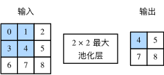
Figure 6 maximum pooling with 2 x 2 window shape

The principle of 2D average pooling is similar to 2D maximum pooling, but the maximum operator is replaced by the average operator. The pool layer whose pool window shape is p × qp × q is called P × qp × Q pool layer, and the pool operation is called P × qp × Q pool.

The pooling layer can also fill in and adjust the window's moving steps on both sides of the input height and width to change the output shape. The mechanism of pool layer filling and stride is the same as that of convolution layer filling and stride.

When processing multi-channel input data, the pooling layer pools each input channel separately, but does not add the results of each channel by channel as the convolution layer does. This means that the number of output channels in the pooling layer is equal to the number of input channels.

2. Classic model

LeNet-5

1998, LeNet5 by Yann LeCun Official website

Although the sparrow is small, it has five internal organs. Convolution layer, pooling layer and full connection layer are the basic components of modern CNN

Spatial features are extracted by convolution;
Sub samples are obtained by space averaging;
tanh or sigmoid are used to obtain nonlinearity;
Multi layer network (MLP) is used as the final classifier;
Sparse connection matrix is used between layers to avoid large calculation cost.

Input: the image Size is 3232. This is larger than the largest letter (2828) in the mnist database. The purpose of this method is to hope that the potential obvious features, such as intermittent strokes and corner points, can appear in the center of the receptive field of the feature monitor at the highest level.

Output: 10 categories, 0-9-digit probability respectively

The C1 layer is a convolution layer, which has six convolution kernels (extracting six local features), and the kernel size is 5 * 5
S2 layer is pooling layer, and lower sampling (area: 2 * 2) reduces the over fitting degree of network training parameters and model.
C3 layer is the second convolution layer, which uses 16 convolution kernels with a kernel size of 5 * 5 to extract features
S4 layer is also a pooling layer, area: 2 * 2
C5 is the last convolution layer, convolution kernel size: 5 * 5 convolution kernel type: 120
Finally, 120 features of C5 are classified by using full connection layer, and the probability of 0-9 is output

Here's the code from Official course

import torch.nn as nn
class LeNet5(nn.Module):

    def __init__(self):
        super(LeNet5, self).__init__()
        # 1 input image channel, 6 output channels, 5x5 square convolution
        # kernel
        self.conv1 = nn.Conv2d(1, 6, 5)
        self.conv2 = nn.Conv2d(6, 16, 5)
        # an affine operation: y = Wx + b
        self.fc1 = nn.Linear(16 * 5 * 5, 120) # The paper here is conv, and the official tutorial uses the linear layer
        self.fc2 = nn.Linear(120, 84)
        self.fc3 = nn.Linear(84, 10)

    def forward(self, x):
        # Max pooling over a (2, 2) window
        x = F.max_pool2d(F.relu(self.conv1(x)), (2, 2))
        # If the size is a square you can only specify a single number
        x = F.max_pool2d(F.relu(self.conv2(x)), 2)
        x = x.view(-1, self.num_flat_features(x))
        x = F.relu(self.fc1(x))
        x = F.relu(self.fc2(x))
        x = self.fc3(x)
        return x

    def num_flat_features(self, x):
        size = x.size()[1:]  # all dimensions except the batch dimension
        num_features = 1
        for s in size:
            num_features *= s
        return num_features


net = LeNet5()
print(net)
LeNet5(
  (conv1): Conv2d(1, 6, kernel_size=(5, 5), stride=(1, 1))
  (conv2): Conv2d(6, 16, kernel_size=(5, 5), stride=(1, 1))
  (fc1): Linear(in_features=400, out_features=120, bias=True)
  (fc2): Linear(in_features=120, out_features=84, bias=True)
  (fc3): Linear(in_features=84, out_features=10, bias=True)
)

AlexNet

2012，Alex Krizhevsky
It can be counted as a deeper and broader version of LeNet, which can be used to learn more complex objects paper

The nonlinearity is obtained by using the corrected linear units (ReLU);
dropout technique is used to selectively ignore single neuron during training to slow down the over fitting of the model;
Overlapping the largest pool to avoid the average effect of the average pool;
Each stage of Alexnet (including one layer of convolution main calculation) can be divided into 8 layers:

The vision package of Python contains the official implementation of Alexnet. We can directly use the official version to look at the network

import torchvision
model = torchvision.models.alexnet(pretrained=False) #We don't download pre training weights
print(model)
AlexNet(
  (features): Sequential(
    (0): Conv2d(3, 64, kernel_size=(11, 11), stride=(4, 4), padding=(2, 2))
    (1): ReLU(inplace)
    (2): MaxPool2d(kernel_size=3, stride=2, padding=0, dilation=1, ceil_mode=False)
    (3): Conv2d(64, 192, kernel_size=(5, 5), stride=(1, 1), padding=(2, 2))
    (4): ReLU(inplace)
    (5): MaxPool2d(kernel_size=3, stride=2, padding=0, dilation=1, ceil_mode=False)
    (6): Conv2d(192, 384, kernel_size=(3, 3), stride=(1, 1), padding=(1, 1))
    (7): ReLU(inplace)
    (8): Conv2d(384, 256, kernel_size=(3, 3), stride=(1, 1), padding=(1, 1))
    (9): ReLU(inplace)
    (10): Conv2d(256, 256, kernel_size=(3, 3), stride=(1, 1), padding=(1, 1))
    (11): ReLU(inplace)
    (12): MaxPool2d(kernel_size=3, stride=2, padding=0, dilation=1, ceil_mode=False)
  )
  (classifier): Sequential(
    (0): Dropout(p=0.5)
    (1): Linear(in_features=9216, out_features=4096, bias=True)
    (2): ReLU(inplace)
    (3): Dropout(p=0.5)
    (4): Linear(in_features=4096, out_features=4096, bias=True)
    (5): ReLU(inplace)
    (6): Linear(in_features=4096, out_features=1000, bias=True)
  )
)

VGG

2015, VGG in Oxford. paper

Use smaller 3 × 3 filters in each convolution layer and combine them into convolution sequence
Multiple 3 × 3 convolution sequences can simulate the effect of larger receiving field
The number of convolution kernels doubles with each time the image pixels are reduced

There are many versions of VGG, which is also a relatively stable and classic model. Its characteristic is continuous conv with large amount of computation. Here we take VGG16 as an example picture source

The advantages of small convolution kernel over large convolution kernel in VGG are summarized in this paper

According to the author's point of view, output=2 after input8 - > 3-layer conv3x3, which is equivalent to the result of 1-layer conv7x7; output=2 after input8 - > 2-layer conv3x3, which is equivalent to the result of 2-layer conv5x5

The parameters of convolution layer are reduced. Compared with the large convolution cores of 5x5, 7x7 and 11x11, 3x3 significantly reduces the parameter amount

After convolution and pooling, the resolution of the image is reduced to half of the original resolution, but the image features are doubled, which is a very regular operation
The resolution is determined by 224 - > 112 - > 56 - > 28 - > 14 - > 7,
Features from original RGB3 channels - > 64 - > 128 - > 256 - > 512

This provides a standard for the later networks. We still use the official version of Python to view it

import torchvision
model = torchvision.models.vgg16(pretrained=False) #We don't download pre training weights
print(model)
VGG(
  (features): Sequential(
    (0): Conv2d(3, 64, kernel_size=(3, 3), stride=(1, 1), padding=(1, 1))
    (1): ReLU(inplace)
    (2): Conv2d(64, 64, kernel_size=(3, 3), stride=(1, 1), padding=(1, 1))
    (3): ReLU(inplace)
    (4): MaxPool2d(kernel_size=2, stride=2, padding=0, dilation=1, ceil_mode=False)
    (5): Conv2d(64, 128, kernel_size=(3, 3), stride=(1, 1), padding=(1, 1))
    (6): ReLU(inplace)
    (7): Conv2d(128, 128, kernel_size=(3, 3), stride=(1, 1), padding=(1, 1))
    (8): ReLU(inplace)
    (9): MaxPool2d(kernel_size=2, stride=2, padding=0, dilation=1, ceil_mode=False)
    (10): Conv2d(128, 256, kernel_size=(3, 3), stride=(1, 1), padding=(1, 1))
    (11): ReLU(inplace)
    (12): Conv2d(256, 256, kernel_size=(3, 3), stride=(1, 1), padding=(1, 1))
    (13): ReLU(inplace)
    (14): Conv2d(256, 256, kernel_size=(3, 3), stride=(1, 1), padding=(1, 1))
    (15): ReLU(inplace)
    (16): MaxPool2d(kernel_size=2, stride=2, padding=0, dilation=1, ceil_mode=False)
    (17): Conv2d(256, 512, kernel_size=(3, 3), stride=(1, 1), padding=(1, 1))
    (18): ReLU(inplace)
    (19): Conv2d(512, 512, kernel_size=(3, 3), stride=(1, 1), padding=(1, 1))
    (20): ReLU(inplace)
    (21): Conv2d(512, 512, kernel_size=(3, 3), stride=(1, 1), padding=(1, 1))
    (22): ReLU(inplace)
    (23): MaxPool2d(kernel_size=2, stride=2, padding=0, dilation=1, ceil_mode=False)
    (24): Conv2d(512, 512, kernel_size=(3, 3), stride=(1, 1), padding=(1, 1))
    (25): ReLU(inplace)
    (26): Conv2d(512, 512, kernel_size=(3, 3), stride=(1, 1), padding=(1, 1))
    (27): ReLU(inplace)
    (28): Conv2d(512, 512, kernel_size=(3, 3), stride=(1, 1), padding=(1, 1))
    (29): ReLU(inplace)
    (30): MaxPool2d(kernel_size=2, stride=2, padding=0, dilation=1, ceil_mode=False)
  )
  (classifier): Sequential(
    (0): Linear(in_features=25088, out_features=4096, bias=True)
    (1): ReLU(inplace)
    (2): Dropout(p=0.5)
    (3): Linear(in_features=4096, out_features=4096, bias=True)
    (4): ReLU(inplace)
    (5): Dropout(p=0.5)
    (6): Linear(in_features=4096, out_features=1000, bias=True)
  )
)

GoogLeNet (Inception)

2014，Google Christian Szegedy paper

Using 1 × 1 convolution block (NiN) to reduce the number of features, which is often called "bottleneck", can reduce the computational burden of deep neural network.
Before each pooling layer, increase feature maps and the width of each layer to increase the combination of features

The biggest feature of Google net is that it contains several inception modules, so it is sometimes called inception net
Although the number of layers of Google net is much more than that of VGG, due to the design of inception, the computing speed is much faster.

Don't be intimidated by this picture. The principle is very simple

The main idea of concept architecture is to find out how to make the existing dense components approach and cover the best local sparse structure in convolutional vision network. Now we need to find the optimal local structure and repeat it several times. In the previous literature, a layer to layer structure was proposed, and correlation statistics were conducted at the last layer to gather high correlation. These clusters form the cells of the next layer and are connected with the cells of the previous layer. Each unit of the front layer is assumed to correspond to certain areas of the input image, which are divided into filter banks. In the lower layer near the input layer, the relevant units are concentrated in some local areas, and finally a large number of clusters in a single area are obtained, which are covered by 1x1 convolution in the last layer.

The first mock exam is very rigid, but it is very simple to explain: every module we use several different feature extraction methods, such as 3x3 convolution, 5x5 convolution, 1x1 convolution, pooling, etc., all of these are calculated, and finally these results are connected through Filter Concat to find the most effective. There are many modules in the network, so we don't need to judge which feature extraction method is good. The network will solve it by itself (it's a bit like AUTO ML). In Python, it implements the concept A-E and the concept aux module.

# Inception? V3 requires scipy, so if it is not installed, pip install scipy
import torchvision
model = torchvision.models.inception_v3(pretrained=False) #We don't download pre training weights
print(model)
Inception3(
  (Conv2d_1a_3x3): BasicConv2d(
    (conv): Conv2d(3, 32, kernel_size=(3, 3), stride=(2, 2), bias=False)
    (bn): BatchNorm2d(32, eps=0.001, momentum=0.1, affine=True, track_running_stats=True)
  )
  (Conv2d_2a_3x3): BasicConv2d(
    (conv): Conv2d(32, 32, kernel_size=(3, 3), stride=(1, 1), bias=False)
    (bn): BatchNorm2d(32, eps=0.001, momentum=0.1, affine=True, track_running_stats=True)
  )
  (Conv2d_2b_3x3): BasicConv2d(
    (conv): Conv2d(32, 64, kernel_size=(3, 3), stride=(1, 1), padding=(1, 1), bias=False)
    (bn): BatchNorm2d(64, eps=0.001, momentum=0.1, affine=True, track_running_stats=True)
  )
  (Conv2d_3b_1x1): BasicConv2d(
    (conv): Conv2d(64, 80, kernel_size=(1, 1), stride=(1, 1), bias=False)
    (bn): BatchNorm2d(80, eps=0.001, momentum=0.1, affine=True, track_running_stats=True)
  )
  (Conv2d_4a_3x3): BasicConv2d(
    (conv): Conv2d(80, 192, kernel_size=(3, 3), stride=(1, 1), bias=False)
    (bn): BatchNorm2d(192, eps=0.001, momentum=0.1, affine=True, track_running_stats=True)
  )
  (Mixed_5b): InceptionA(
    (branch1x1): BasicConv2d(
      (conv): Conv2d(192, 64, kernel_size=(1, 1), stride=(1, 1), bias=False)
      (bn): BatchNorm2d(64, eps=0.001, momentum=0.1, affine=True, track_running_stats=True)
    )
    (branch5x5_1): BasicConv2d(
      (conv): Conv2d(192, 48, kernel_size=(1, 1), stride=(1, 1), bias=False)
      (bn): BatchNorm2d(48, eps=0.001, momentum=0.1, affine=True, track_running_stats=True)
    )
    (branch5x5_2): BasicConv2d(
      (conv): Conv2d(48, 64, kernel_size=(5, 5), stride=(1, 1), padding=(2, 2), bias=False)
      (bn): BatchNorm2d(64, eps=0.001, momentum=0.1, affine=True, track_running_stats=True)
    )
    (branch3x3dbl_1): BasicConv2d(
      (conv): Conv2d(192, 64, kernel_size=(1, 1), stride=(1, 1), bias=False)
      (bn): BatchNorm2d(64, eps=0.001, momentum=0.1, affine=True, track_running_stats=True)
    )
    (branch3x3dbl_2): BasicConv2d(
      (conv): Conv2d(64, 96, kernel_size=(3, 3), stride=(1, 1), padding=(1, 1), bias=False)
      (bn): BatchNorm2d(96, eps=0.001, momentum=0.1, affine=True, track_running_stats=True)
    )
    (branch3x3dbl_3): BasicConv2d(
      (conv): Conv2d(96, 96, kernel_size=(3, 3), stride=(1, 1), padding=(1, 1), bias=False)
      (bn): BatchNorm2d(96, eps=0.001, momentum=0.1, affine=True, track_running_stats=True)
    )
    (branch_pool): BasicConv2d(
      (conv): Conv2d(192, 32, kernel_size=(1, 1), stride=(1, 1), bias=False)
      (bn): BatchNorm2d(32, eps=0.001, momentum=0.1, affine=True, track_running_stats=True)
    )
  )
  (Mixed_5c): InceptionA(
    (branch1x1): BasicConv2d(
      (conv): Conv2d(256, 64, kernel_size=(1, 1), stride=(1, 1), bias=False)
      (bn): BatchNorm2d(64, eps=0.001, momentum=0.1, affine=True, track_running_stats=True)
    )
    (branch5x5_1): BasicConv2d(
      (conv): Conv2d(256, 48, kernel_size=(1, 1), stride=(1, 1), bias=False)
      (bn): BatchNorm2d(48, eps=0.001, momentum=0.1, affine=True, track_running_stats=True)
    )
    (branch5x5_2): BasicConv2d(
      (conv): Conv2d(48, 64, kernel_size=(5, 5), stride=(1, 1), padding=(2, 2), bias=False)
      (bn): BatchNorm2d(64, eps=0.001, momentum=0.1, affine=True, track_running_stats=True)
    )
    (branch3x3dbl_1): BasicConv2d(
      (conv): Conv2d(256, 64, kernel_size=(1, 1), stride=(1, 1), bias=False)
      (bn): BatchNorm2d(64, eps=0.001, momentum=0.1, affine=True, track_running_stats=True)
    )
    (branch3x3dbl_2): BasicConv2d(
      (conv): Conv2d(64, 96, kernel_size=(3, 3), stride=(1, 1), padding=(1, 1), bias=False)
      (bn): BatchNorm2d(96, eps=0.001, momentum=0.1, affine=True, track_running_stats=True)
    )
    (branch3x3dbl_3): BasicConv2d(
      (conv): Conv2d(96, 96, kernel_size=(3, 3), stride=(1, 1), padding=(1, 1), bias=False)
      (bn): BatchNorm2d(96, eps=0.001, momentum=0.1, affine=True, track_running_stats=True)
    )
    (branch_pool): BasicConv2d(
      (conv): Conv2d(256, 64, kernel_size=(1, 1), stride=(1, 1), bias=False)
      (bn): BatchNorm2d(64, eps=0.001, momentum=0.1, affine=True, track_running_stats=True)
    )
  )
  (Mixed_5d): InceptionA(
    (branch1x1): BasicConv2d(
      (conv): Conv2d(288, 64, kernel_size=(1, 1), stride=(1, 1), bias=False)
      (bn): BatchNorm2d(64, eps=0.001, momentum=0.1, affine=True, track_running_stats=True)
    )
    (branch5x5_1): BasicConv2d(
      (conv): Conv2d(288, 48, kernel_size=(1, 1), stride=(1, 1), bias=False)
      (bn): BatchNorm2d(48, eps=0.001, momentum=0.1, affine=True, track_running_stats=True)
    )
    (branch5x5_2): BasicConv2d(
      (conv): Conv2d(48, 64, kernel_size=(5, 5), stride=(1, 1), padding=(2, 2), bias=False)
      (bn): BatchNorm2d(64, eps=0.001, momentum=0.1, affine=True, track_running_stats=True)
    )
    (branch3x3dbl_1): BasicConv2d(
      (conv): Conv2d(288, 64, kernel_size=(1, 1), stride=(1, 1), bias=False)
      (bn): BatchNorm2d(64, eps=0.001, momentum=0.1, affine=True, track_running_stats=True)
    )
    (branch3x3dbl_2): BasicConv2d(
      (conv): Conv2d(64, 96, kernel_size=(3, 3), stride=(1, 1), padding=(1, 1), bias=False)
      (bn): BatchNorm2d(96, eps=0.001, momentum=0.1, affine=True, track_running_stats=True)
    )
    (branch3x3dbl_3): BasicConv2d(
      (conv): Conv2d(96, 96, kernel_size=(3, 3), stride=(1, 1), padding=(1, 1), bias=False)
      (bn): BatchNorm2d(96, eps=0.001, momentum=0.1, affine=True, track_running_stats=True)
    )
    (branch_pool): BasicConv2d(
      (conv): Conv2d(288, 64, kernel_size=(1, 1), stride=(1, 1), bias=False)
      (bn): BatchNorm2d(64, eps=0.001, momentum=0.1, affine=True, track_running_stats=True)
    )
  )
  (Mixed_6a): InceptionB(
    (branch3x3): BasicConv2d(
      (conv): Conv2d(288, 384, kernel_size=(3, 3), stride=(2, 2), bias=False)
      (bn): BatchNorm2d(384, eps=0.001, momentum=0.1, affine=True, track_running_stats=True)
    )
    (branch3x3dbl_1): BasicConv2d(
      (conv): Conv2d(288, 64, kernel_size=(1, 1), stride=(1, 1), bias=False)
      (bn): BatchNorm2d(64, eps=0.001, momentum=0.1, affine=True, track_running_stats=True)
    )
    (branch3x3dbl_2): BasicConv2d(
      (conv): Conv2d(64, 96, kernel_size=(3, 3), stride=(1, 1), padding=(1, 1), bias=False)
      (bn): BatchNorm2d(96, eps=0.001, momentum=0.1, affine=True, track_running_stats=True)
    )
    (branch3x3dbl_3): BasicConv2d(
      (conv): Conv2d(96, 96, kernel_size=(3, 3), stride=(2, 2), bias=False)
      (bn): BatchNorm2d(96, eps=0.001, momentum=0.1, affine=True, track_running_stats=True)
    )
  )
  (Mixed_6b): InceptionC(
    (branch1x1): BasicConv2d(
      (conv): Conv2d(768, 192, kernel_size=(1, 1), stride=(1, 1), bias=False)
      (bn): BatchNorm2d(192, eps=0.001, momentum=0.1, affine=True, track_running_stats=True)
    )
    (branch7x7_1): BasicConv2d(
      (conv): Conv2d(768, 128, kernel_size=(1, 1), stride=(1, 1), bias=False)
      (bn): BatchNorm2d(128, eps=0.001, momentum=0.1, affine=True, track_running_stats=True)
    )
    (branch7x7_2): BasicConv2d(
      (conv): Conv2d(128, 128, kernel_size=(1, 7), stride=(1, 1), padding=(0, 3), bias=False)
      (bn): BatchNorm2d(128, eps=0.001, momentum=0.1, affine=True, track_running_stats=True)
    )
    (branch7x7_3): BasicConv2d(
      (conv): Conv2d(128, 192, kernel_size=(7, 1), stride=(1, 1), padding=(3, 0), bias=False)
      (bn): BatchNorm2d(192, eps=0.001, momentum=0.1, affine=True, track_running_stats=True)
    )
    (branch7x7dbl_1): BasicConv2d(
      (conv): Conv2d(768, 128, kernel_size=(1, 1), stride=(1, 1), bias=False)
      (bn): BatchNorm2d(128, eps=0.001, momentum=0.1, affine=True, track_running_stats=True)
    )
    (branch7x7dbl_2): BasicConv2d(
      (conv): Conv2d(128, 128, kernel_size=(7, 1), stride=(1, 1), padding=(3, 0), bias=False)
      (bn): BatchNorm2d(128, eps=0.001, momentum=0.1, affine=True, track_running_stats=True)
    )
    (branch7x7dbl_3): BasicConv2d(
      (conv): Conv2d(128, 128, kernel_size=(1, 7), stride=(1, 1), padding=(0, 3), bias=False)
      (bn): BatchNorm2d(128, eps=0.001, momentum=0.1, affine=True, track_running_stats=True)
    )
    (branch7x7dbl_4): BasicConv2d(
      (conv): Conv2d(128, 128, kernel_size=(7, 1), stride=(1, 1), padding=(3, 0), bias=False)
      (bn): BatchNorm2d(128, eps=0.001, momentum=0.1, affine=True, track_running_stats=True)
    )
    (branch7x7dbl_5): BasicConv2d(
      (conv): Conv2d(128, 192, kernel_size=(1, 7), stride=(1, 1), padding=(0, 3), bias=False)
      (bn): BatchNorm2d(192, eps=0.001, momentum=0.1, affine=True, track_running_stats=True)
    )
    (branch_pool): BasicConv2d(
      (conv): Conv2d(768, 192, kernel_size=(1, 1), stride=(1, 1), bias=False)
      (bn): BatchNorm2d(192, eps=0.001, momentum=0.1, affine=True, track_running_stats=True)
    )
  )
  (Mixed_6c): InceptionC(
    (branch1x1): BasicConv2d(
      (conv): Conv2d(768, 192, kernel_size=(1, 1), stride=(1, 1), bias=False)
      (bn): BatchNorm2d(192, eps=0.001, momentum=0.1, affine=True, track_running_stats=True)
    )
    (branch7x7_1): BasicConv2d(
      (conv): Conv2d(768, 160, kernel_size=(1, 1), stride=(1, 1), bias=False)
      (bn): BatchNorm2d(160, eps=0.001, momentum=0.1, affine=True, track_running_stats=True)
    )
    (branch7x7_2): BasicConv2d(
      (conv): Conv2d(160, 160, kernel_size=(1, 7), stride=(1, 1), padding=(0, 3), bias=False)
      (bn): BatchNorm2d(160, eps=0.001, momentum=0.1, affine=True, track_running_stats=True)
    )
    (branch7x7_3): BasicConv2d(
      (conv): Conv2d(160, 192, kernel_size=(7, 1), stride=(1, 1), padding=(3, 0), bias=False)
      (bn): BatchNorm2d(192, eps=0.001, momentum=0.1, affine=True, track_running_stats=True)
    )
    (branch7x7dbl_1): BasicConv2d(
      (conv): Conv2d(768, 160, kernel_size=(1, 1), stride=(1, 1), bias=False)
      (bn): BatchNorm2d(160, eps=0.001, momentum=0.1, affine=True, track_running_stats=True)
    )
    (branch7x7dbl_2): BasicConv2d(
      (conv): Conv2d(160, 160, kernel_size=(7, 1), stride=(1, 1), padding=(3, 0), bias=False)
      (bn): BatchNorm2d(160, eps=0.001, momentum=0.1, affine=True, track_running_stats=True)
    )
    (branch7x7dbl_3): BasicConv2d(
      (conv): Conv2d(160, 160, kernel_size=(1, 7), stride=(1, 1), padding=(0, 3), bias=False)
      (bn): BatchNorm2d(160, eps=0.001, momentum=0.1, affine=True, track_running_stats=True)
    )
    (branch7x7dbl_4): BasicConv2d(
      (conv): Conv2d(160, 160, kernel_size=(7, 1), stride=(1, 1), padding=(3, 0), bias=False)
      (bn): BatchNorm2d(160, eps=0.001, momentum=0.1, affine=True, track_running_stats=True)
    )
    (branch7x7dbl_5): BasicConv2d(
      (conv): Conv2d(160, 192, kernel_size=(1, 7), stride=(1, 1), padding=(0, 3), bias=False)
      (bn): BatchNorm2d(192, eps=0.001, momentum=0.1, affine=True, track_running_stats=True)
    )
    (branch_pool): BasicConv2d(
      (conv): Conv2d(768, 192, kernel_size=(1, 1), stride=(1, 1), bias=False)
      (bn): BatchNorm2d(192, eps=0.001, momentum=0.1, affine=True, track_running_stats=True)
    )
  )
  (Mixed_6d): InceptionC(
    (branch1x1): BasicConv2d(
      (conv): Conv2d(768, 192, kernel_size=(1, 1), stride=(1, 1), bias=False)
      (bn): BatchNorm2d(192, eps=0.001, momentum=0.1, affine=True, track_running_stats=True)
    )
    (branch7x7_1): BasicConv2d(
      (conv): Conv2d(768, 160, kernel_size=(1, 1), stride=(1, 1), bias=False)
      (bn): BatchNorm2d(160, eps=0.001, momentum=0.1, affine=True, track_running_stats=True)
    )
    (branch7x7_2): BasicConv2d(
      (conv): Conv2d(160, 160, kernel_size=(1, 7), stride=(1, 1), padding=(0, 3), bias=False)
      (bn): BatchNorm2d(160, eps=0.001, momentum=0.1, affine=True, track_running_stats=True)
    )
    (branch7x7_3): BasicConv2d(
      (conv): Conv2d(160, 192, kernel_size=(7, 1), stride=(1, 1), padding=(3, 0), bias=False)
      (bn): BatchNorm2d(192, eps=0.001, momentum=0.1, affine=True, track_running_stats=True)
    )
    (branch7x7dbl_1): BasicConv2d(
      (conv): Conv2d(768, 160, kernel_size=(1, 1), stride=(1, 1), bias=False)
      (bn): BatchNorm2d(160, eps=0.001, momentum=0.1, affine=True, track_running_stats=True)
    )
    (branch7x7dbl_2): BasicConv2d(
      (conv): Conv2d(160, 160, kernel_size=(7, 1), stride=(1, 1), padding=(3, 0), bias=False)
      (bn): BatchNorm2d(160, eps=0.001, momentum=0.1, affine=True, track_running_stats=True)
    )
    (branch7x7dbl_3): BasicConv2d(
      (conv): Conv2d(160, 160, kernel_size=(1, 7), stride=(1, 1), padding=(0, 3), bias=False)
      (bn): BatchNorm2d(160, eps=0.001, momentum=0.1, affine=True, track_running_stats=True)
    )
    (branch7x7dbl_4): BasicConv2d(
      (conv): Conv2d(160, 160, kernel_size=(7, 1), stride=(1, 1), padding=(3, 0), bias=False)
      (bn): BatchNorm2d(160, eps=0.001, momentum=0.1, affine=True, track_running_stats=True)
    )
    (branch7x7dbl_5): BasicConv2d(
      (conv): Conv2d(160, 192, kernel_size=(1, 7), stride=(1, 1), padding=(0, 3), bias=False)
      (bn): BatchNorm2d(192, eps=0.001, momentum=0.1, affine=True, track_running_stats=True)
    )
    (branch_pool): BasicConv2d(
      (conv): Conv2d(768, 192, kernel_size=(1, 1), stride=(1, 1), bias=False)
      (bn): BatchNorm2d(192, eps=0.001, momentum=0.1, affine=True, track_running_stats=True)
    )
  )
  (Mixed_6e): InceptionC(
    (branch1x1): BasicConv2d(
      (conv): Conv2d(768, 192, kernel_size=(1, 1), stride=(1, 1), bias=False)
      (bn): BatchNorm2d(192, eps=0.001, momentum=0.1, affine=True, track_running_stats=True)
    )
    (branch7x7_1): BasicConv2d(
      (conv): Conv2d(768, 192, kernel_size=(1, 1), stride=(1, 1), bias=False)
      (bn): BatchNorm2d(192, eps=0.001, momentum=0.1, affine=True, track_running_stats=True)
    )
    (branch7x7_2): BasicConv2d(
      (conv): Conv2d(192, 192, kernel_size=(1, 7), stride=(1, 1), padding=(0, 3), bias=False)
      (bn): BatchNorm2d(192, eps=0.001, momentum=0.1, affine=True, track_running_stats=True)
    )
    (branch7x7_3): BasicConv2d(
      (conv): Conv2d(192, 192, kernel_size=(7, 1), stride=(1, 1), padding=(3, 0), bias=False)
      (bn): BatchNorm2d(192, eps=0.001, momentum=0.1, affine=True, track_running_stats=True)
    )
    (branch7x7dbl_1): BasicConv2d(
      (conv): Conv2d(768, 192, kernel_size=(1, 1), stride=(1, 1), bias=False)
      (bn): BatchNorm2d(192, eps=0.001, momentum=0.1, affine=True, track_running_stats=True)
    )
    (branch7x7dbl_2): BasicConv2d(
      (conv): Conv2d(192, 192, kernel_size=(7, 1), stride=(1, 1), padding=(3, 0), bias=False)
      (bn): BatchNorm2d(192, eps=0.001, momentum=0.1, affine=True, track_running_stats=True)
    )
    (branch7x7dbl_3): BasicConv2d(
      (conv): Conv2d(192, 192, kernel_size=(1, 7), stride=(1, 1), padding=(0, 3), bias=False)
      (bn): BatchNorm2d(192, eps=0.001, momentum=0.1, affine=True, track_running_stats=True)
    )
    (branch7x7dbl_4): BasicConv2d(
      (conv): Conv2d(192, 192, kernel_size=(7, 1), stride=(1, 1), padding=(3, 0), bias=False)
      (bn): BatchNorm2d(192, eps=0.001, momentum=0.1, affine=True, track_running_stats=True)
    )
    (branch7x7dbl_5): BasicConv2d(
      (conv): Conv2d(192, 192, kernel_size=(1, 7), stride=(1, 1), padding=(0, 3), bias=False)
      (bn): BatchNorm2d(192, eps=0.001, momentum=0.1, affine=True, track_running_stats=True)
    )
    (branch_pool): BasicConv2d(
      (conv): Conv2d(768, 192, kernel_size=(1, 1), stride=(1, 1), bias=False)
      (bn): BatchNorm2d(192, eps=0.001, momentum=0.1, affine=True, track_running_stats=True)
    )
  )
  (AuxLogits): InceptionAux(
    (conv0): BasicConv2d(
      (conv): Conv2d(768, 128, kernel_size=(1, 1), stride=(1, 1), bias=False)
      (bn): BatchNorm2d(128, eps=0.001, momentum=0.1, affine=True, track_running_stats=True)
    )
    (conv1): BasicConv2d(
      (conv): Conv2d(128, 768, kernel_size=(5, 5), stride=(1, 1), bias=False)
      (bn): BatchNorm2d(768, eps=0.001, momentum=0.1, affine=True, track_running_stats=True)
    )
    (fc): Linear(in_features=768, out_features=1000, bias=True)
  )
  (Mixed_7a): InceptionD(
    (branch3x3_1): BasicConv2d(
      (conv): Conv2d(768, 192, kernel_size=(1, 1), stride=(1, 1), bias=False)
      (bn): BatchNorm2d(192, eps=0.001, momentum=0.1, affine=True, track_running_stats=True)
    )
    (branch3x3_2): BasicConv2d(
      (conv): Conv2d(192, 320, kernel_size=(3, 3), stride=(2, 2), bias=False)
      (bn): BatchNorm2d(320, eps=0.001, momentum=0.1, affine=True, track_running_stats=True)
    )
    (branch7x7x3_1): BasicConv2d(
      (conv): Conv2d(768, 192, kernel_size=(1, 1), stride=(1, 1), bias=False)
      (bn): BatchNorm2d(192, eps=0.001, momentum=0.1, affine=True, track_running_stats=True)
    )
    (branch7x7x3_2): BasicConv2d(
      (conv): Conv2d(192, 192, kernel_size=(1, 7), stride=(1, 1), padding=(0, 3), bias=False)
      (bn): BatchNorm2d(192, eps=0.001, momentum=0.1, affine=True, track_running_stats=True)
    )
    (branch7x7x3_3): BasicConv2d(
      (conv): Conv2d(192, 192, kernel_size=(7, 1), stride=(1, 1), padding=(3, 0), bias=False)
      (bn): BatchNorm2d(192, eps=0.001, momentum=0.1, affine=True, track_running_stats=True)
    )
    (branch7x7x3_4): BasicConv2d(
      (conv): Conv2d(192, 192, kernel_size=(3, 3), stride=(2, 2), bias=False)
      (bn): BatchNorm2d(192, eps=0.001, momentum=0.1, affine=True, track_running_stats=True)
    )
  )
  (Mixed_7b): InceptionE(
    (branch1x1): BasicConv2d(
      (conv): Conv2d(1280, 320, kernel_size=(1, 1), stride=(1, 1), bias=False)
      (bn): BatchNorm2d(320, eps=0.001, momentum=0.1, affine=True, track_running_stats=True)
    )
    (branch3x3_1): BasicConv2d(
      (conv): Conv2d(1280, 384, kernel_size=(1, 1), stride=(1, 1), bias=False)
      (bn): BatchNorm2d(384, eps=0.001, momentum=0.1, affine=True, track_running_stats=True)
    )
    (branch3x3_2a): BasicConv2d(
      (conv): Conv2d(384, 384, kernel_size=(1, 3), stride=(1, 1), padding=(0, 1), bias=False)
      (bn): BatchNorm2d(384, eps=0.001, momentum=0.1, affine=True, track_running_stats=True)
    )
    (branch3x3_2b): BasicConv2d(
      (conv): Conv2d(384, 384, kernel_size=(3, 1), stride=(1, 1), padding=(1, 0), bias=False)
      (bn): BatchNorm2d(384, eps=0.001, momentum=0.1, affine=True, track_running_stats=True)
    )
    (branch3x3dbl_1): BasicConv2d(
      (conv): Conv2d(1280, 448, kernel_size=(1, 1), stride=(1, 1), bias=False)
      (bn): BatchNorm2d(448, eps=0.001, momentum=0.1, affine=True, track_running_stats=True)
    )
    (branch3x3dbl_2): BasicConv2d(
      (conv): Conv2d(448, 384, kernel_size=(3, 3), stride=(1, 1), padding=(1, 1), bias=False)
      (bn): BatchNorm2d(384, eps=0.001, momentum=0.1, affine=True, track_running_stats=True)
    )
    (branch3x3dbl_3a): BasicConv2d(
      (conv): Conv2d(384, 384, kernel_size=(1, 3), stride=(1, 1), padding=(0, 1), bias=False)
      (bn): BatchNorm2d(384, eps=0.001, momentum=0.1, affine=True, track_running_stats=True)
    )
    (branch3x3dbl_3b): BasicConv2d(
      (conv): Conv2d(384, 384, kernel_size=(3, 1), stride=(1, 1), padding=(1, 0), bias=False)
      (bn): BatchNorm2d(384, eps=0.001, momentum=0.1, affine=True, track_running_stats=True)
    )
    (branch_pool): BasicConv2d(
      (conv): Conv2d(1280, 192, kernel_size=(1, 1), stride=(1, 1), bias=False)
      (bn): BatchNorm2d(192, eps=0.001, momentum=0.1, affine=True, track_running_stats=True)
    )
  )
  (Mixed_7c): InceptionE(
    (branch1x1): BasicConv2d(
      (conv): Conv2d(2048, 320, kernel_size=(1, 1), stride=(1, 1), bias=False)
      (bn): BatchNorm2d(320, eps=0.001, momentum=0.1, affine=True, track_running_stats=True)
    )
    (branch3x3_1): BasicConv2d(
      (conv): Conv2d(2048, 384, kernel_size=(1, 1), stride=(1, 1), bias=False)
      (bn): BatchNorm2d(384, eps=0.001, momentum=0.1, affine=True, track_running_stats=True)
    )
    (branch3x3_2a): BasicConv2d(
      (conv): Conv2d(384, 384, kernel_size=(1, 3), stride=(1, 1), padding=(0, 1), bias=False)
      (bn): BatchNorm2d(384, eps=0.001, momentum=0.1, affine=True, track_running_stats=True)
    )
    (branch3x3_2b): BasicConv2d(
      (conv): Conv2d(384, 384, kernel_size=(3, 1), stride=(1, 1), padding=(1, 0), bias=False)
      (bn): BatchNorm2d(384, eps=0.001, momentum=0.1, affine=True, track_running_stats=True)
    )
    (branch3x3dbl_1): BasicConv2d(
      (conv): Conv2d(2048, 448, kernel_size=(1, 1), stride=(1, 1), bias=False)
      (bn): BatchNorm2d(448, eps=0.001, momentum=0.1, affine=True, track_running_stats=True)
    )
    (branch3x3dbl_2): BasicConv2d(
      (conv): Conv2d(448, 384, kernel_size=(3, 3), stride=(1, 1), padding=(1, 1), bias=False)
      (bn): BatchNorm2d(384, eps=0.001, momentum=0.1, affine=True, track_running_stats=True)
    )
    (branch3x3dbl_3a): BasicConv2d(
      (conv): Conv2d(384, 384, kernel_size=(1, 3), stride=(1, 1), padding=(0, 1), bias=False)
      (bn): BatchNorm2d(384, eps=0.001, momentum=0.1, affine=True, track_running_stats=True)
    )
    (branch3x3dbl_3b): BasicConv2d(
      (conv): Conv2d(384, 384, kernel_size=(3, 1), stride=(1, 1), padding=(1, 0), bias=False)
      (bn): BatchNorm2d(384, eps=0.001, momentum=0.1, affine=True, track_running_stats=True)
    )
    (branch_pool): BasicConv2d(
      (conv): Conv2d(2048, 192, kernel_size=(1, 1), stride=(1, 1), bias=False)
      (bn): BatchNorm2d(192, eps=0.001, momentum=0.1, affine=True, track_running_stats=True)
    )
  )
  (fc): Linear(in_features=2048, out_features=1000, bias=True)

ResNet

2015，Kaiming He, Xiangyu Zhang, Shaoqing Ren, Jian Sun paper
Kaiming He is the God of science and technology. You must remember that he is involved in many papers. Let alone Mr. Sun Jian, the chief scientist of Kuangshi technology
The Google net just now is very deep. ResNet can be deeper. Through residual calculation, it can train more than 1000 layers of network, commonly known as jump connection

Degradation problem

The number of network layers increases, but the accuracy of training set is saturated or even decreased. This can't be interpreted as overfitting, because overfit should be better in the training set. This is the problem of network degradation, which shows that deep networks can not be simply optimized

The solution of residual network

If the later layers of the deep network are identity maps, the model will degenerate into a shallow network. Now we have to learn identity mapping function. It is difficult to fit a potential identity mapping function H(x) = x by some layers. If the network is designed as H(x) = F(x) + x. We can transform it into learning a residual function F(x) = H(x) - x. as long as F(x)=0, an identity map H(x) = x. moreover, fitting residual must be easier.

The above is not easy to understand. Continue to explain, first look at the picture:

Before activating the function, we add the output of the previous layer (or layers) and the output calculated by this layer, and input the sum result into the activation function as the output of this layer. The mapping after introducing the residual is more sensitive to the change of the output. In fact, it depends on whether there is a big change in this layer compared with the previous layers, which is equivalent to the function of a differential amplifier. The curve in the figure is the shortcut in the residual. It connects the results of the previous layer directly to the current layer, also known as jump connection.

Let's take a look at the network structure with the classic resnet18

import torchvision
model = torchvision.models.resnet18(pretrained=False) #We don't download pre training weights
print(model)
ResNet(
  (conv1): Conv2d(3, 64, kernel_size=(7, 7), stride=(2, 2), padding=(3, 3), bias=False)
  (bn1): BatchNorm2d(64, eps=1e-05, momentum=0.1, affine=True, track_running_stats=True)
  (relu): ReLU(inplace)
  (maxpool): MaxPool2d(kernel_size=3, stride=2, padding=1, dilation=1, ceil_mode=False)
  (layer1): Sequential(
    (0): BasicBlock(
      (conv1): Conv2d(64, 64, kernel_size=(3, 3), stride=(1, 1), padding=(1, 1), bias=False)
      (bn1): BatchNorm2d(64, eps=1e-05, momentum=0.1, affine=True, track_running_stats=True)
      (relu): ReLU(inplace)
      (conv2): Conv2d(64, 64, kernel_size=(3, 3), stride=(1, 1), padding=(1, 1), bias=False)
      (bn2): BatchNorm2d(64, eps=1e-05, momentum=0.1, affine=True, track_running_stats=True)
    )
    (1): BasicBlock(
      (conv1): Conv2d(64, 64, kernel_size=(3, 3), stride=(1, 1), padding=(1, 1), bias=False)
      (bn1): BatchNorm2d(64, eps=1e-05, momentum=0.1, affine=True, track_running_stats=True)
      (relu): ReLU(inplace)
      (conv2): Conv2d(64, 64, kernel_size=(3, 3), stride=(1, 1), padding=(1, 1), bias=False)
      (bn2): BatchNorm2d(64, eps=1e-05, momentum=0.1, affine=True, track_running_stats=True)
    )
  )
  (layer2): Sequential(
    (0): BasicBlock(
      (conv1): Conv2d(64, 128, kernel_size=(3, 3), stride=(2, 2), padding=(1, 1), bias=False)
      (bn1): BatchNorm2d(128, eps=1e-05, momentum=0.1, affine=True, track_running_stats=True)
      (relu): ReLU(inplace)
      (conv2): Conv2d(128, 128, kernel_size=(3, 3), stride=(1, 1), padding=(1, 1), bias=False)
      (bn2): BatchNorm2d(128, eps=1e-05, momentum=0.1, affine=True, track_running_stats=True)
      (downsample): Sequential(
        (0): Conv2d(64, 128, kernel_size=(1, 1), stride=(2, 2), bias=False)
        (1): BatchNorm2d(128, eps=1e-05, momentum=0.1, affine=True, track_running_stats=True)
      )
    )
    (1): BasicBlock(
      (conv1): Conv2d(128, 128, kernel_size=(3, 3), stride=(1, 1), padding=(1, 1), bias=False)
      (bn1): BatchNorm2d(128, eps=1e-05, momentum=0.1, affine=True, track_running_stats=True)
      (relu): ReLU(inplace)
      (conv2): Conv2d(128, 128, kernel_size=(3, 3), stride=(1, 1), padding=(1, 1), bias=False)
      (bn2): BatchNorm2d(128, eps=1e-05, momentum=0.1, affine=True, track_running_stats=True)
    )
  )
  (layer3): Sequential(
    (0): BasicBlock(
      (conv1): Conv2d(128, 256, kernel_size=(3, 3), stride=(2, 2), padding=(1, 1), bias=False)
      (bn1): BatchNorm2d(256, eps=1e-05, momentum=0.1, affine=True, track_running_stats=True)
      (relu): ReLU(inplace)
      (conv2): Conv2d(256, 256, kernel_size=(3, 3), stride=(1, 1), padding=(1, 1), bias=False)
      (bn2): BatchNorm2d(256, eps=1e-05, momentum=0.1, affine=True, track_running_stats=True)
      (downsample): Sequential(
        (0): Conv2d(128, 256, kernel_size=(1, 1), stride=(2, 2), bias=False)
        (1): BatchNorm2d(256, eps=1e-05, momentum=0.1, affine=True, track_running_stats=True)
      )
    )
    (1): BasicBlock(
      (conv1): Conv2d(256, 256, kernel_size=(3, 3), stride=(1, 1), padding=(1, 1), bias=False)
      (bn1): BatchNorm2d(256, eps=1e-05, momentum=0.1, affine=True, track_running_stats=True)
      (relu): ReLU(inplace)
      (conv2): Conv2d(256, 256, kernel_size=(3, 3), stride=(1, 1), padding=(1, 1), bias=False)
      (bn2): BatchNorm2d(256, eps=1e-05, momentum=0.1, affine=True, track_running_stats=True)
    )
  )
  (layer4): Sequential(
    (0): BasicBlock(
      (conv1): Conv2d(256, 512, kernel_size=(3, 3), stride=(2, 2), padding=(1, 1), bias=False)
      (bn1): BatchNorm2d(512, eps=1e-05, momentum=0.1, affine=True, track_running_stats=True)
      (relu): ReLU(inplace)
      (conv2): Conv2d(512, 512, kernel_size=(3, 3), stride=(1, 1), padding=(1, 1), bias=False)
      (bn2): BatchNorm2d(512, eps=1e-05, momentum=0.1, affine=True, track_running_stats=True)
      (downsample): Sequential(
        (0): Conv2d(256, 512, kernel_size=(1, 1), stride=(2, 2), bias=False)
        (1): BatchNorm2d(512, eps=1e-05, momentum=0.1, affine=True, track_running_stats=True)
      )
    )pypythpn
    (1): BasicBlock(
      (conv1): Conv2d(512, 512, kernel_size=(3, 3), stride=(1, 1), padding=(1, 1), bias=False)
      (bn1): BatchNorm2d(512, eps=1e-05, momentum=0.1, affine=True, track_running_stats=True)
      (relu): ReLU(inplace)
      (conv2): Conv2d(512, 512, kernel_size=(3, 3), stride=(1, 1), padding=(1, 1), bias=False)
      (bn2): BatchNorm2d(512, eps=1e-05, momentum=0.1, affine=True, track_running_stats=True)
    )
  )
  (avgpool): AvgPool2d(kernel_size=7, stride=1, padding=0)
  (fc): Linear(in_features=512, out_features=1000, bias=True)
)

So how do we choose the network?
The above table can clearly see the comparison between accuracy and calculation amount. My suggestion is that resnet18 is basically OK for the small-scale image classification task. If you really need high accuracy, choose another better network architecture.

There is another saying: the poor can only use alexnet, and the rich can use Res.

3. Construction of convolution neural network model

Convolutional Neural Network

You need to import the required package first

import time
import numpy as np
import torch
import torch.nn.functional as F
from torchvision import datasets
from torchvision import transforms
from torch.utils.data import DataLoader
if torch.cuda.is_available():
    torch.backends.cudnn.deterministic = True

Configuration and data processing


# Parameters of related configuration
device = torch.device("cuda:3" if torch.cuda.is_available() else "cpu")

# Hyperparameters
random_seed = 1
learning_rate = 0.05
num_epochs = 10
batch_size = 128

# Importing and partitioning datasets
num_classes = 10
train_dataset = datasets.MNIST(root='data', 
                               train=True, 
                               transform=transforms.ToTensor(),
                               download=True)

test_dataset = datasets.MNIST(root='data', 
                              train=False, 
                              transform=transforms.ToTensor())


train_loader = DataLoader(dataset=train_dataset, 
                          batch_size=batch_size, 
                          shuffle=True)

test_loader = DataLoader(dataset=test_dataset, 
                         batch_size=batch_size, 
                         shuffle=False)

# Checking the dataset
for images, labels in train_loader:  
    print('Image batch dimensions:', images.shape)
    print('Image label dimensions:', labels.shape)
    break

View the details of the data

Image batch dimensions: torch.Size([128, 1, 28, 28])
Image label dimensions: torch.Size([128])

Model building

class ConvNet(torch.nn.Module):

    def __init__(self, num_classes):
        super(ConvNet, self).__init__()
        
        # calculate same padding:
        # (w - k + 2*p)/s + 1 = o
        # => p = (s(o-1) - w + k)/2
        
        # 28x28x1 => 28x28x8
        self.conv_1 = torch.nn.Conv2d(in_channels=1,
                                      out_channels=8,
                                      kernel_size=(3, 3),
                                      stride=(1, 1),
                                      padding=1) # (1(28-1) - 28 + 3) / 2 = 1
        # 28x28x8 => 14x14x8
        self.pool_1 = torch.nn.MaxPool2d(kernel_size=(2, 2),
                                         stride=(2, 2),
                                         padding=0) # (2(14-1) - 28 + 2) = 0                                       
        # 14x14x8 => 14x14x16
        self.conv_2 = torch.nn.Conv2d(in_channels=8,
                                      out_channels=16,
                                      kernel_size=(3, 3),
                                      stride=(1, 1),
                                      padding=1) # (1(14-1) - 14 + 3) / 2 = 1                 
        # 14x14x16 => 7x7x16                             
        self.pool_2 = torch.nn.MaxPool2d(kernel_size=(2, 2),
                                         stride=(2, 2),
                                         padding=0) # (2(7-1) - 14 + 2) = 0

        self.linear_1 = torch.nn.Linear(7*7*16, num_classes)

        # optionally initialize weights from Gaussian;
        # Guassian weight init is not recommended and only for demonstration purposes
        for m in self.modules():
            if isinstance(m, torch.nn.Conv2d) or isinstance(m, torch.nn.Linear):
                m.weight.data.normal_(0.0, 0.01)
                m.bias.data.zero_()
                if m.bias is not None:
                    m.bias.detach().zero_()
        
        
    def forward(self, x):
        out = self.conv_1(x)
        out = F.relu(out)
        out = self.pool_1(out)

        out = self.conv_2(out)
        out = F.relu(out)
        out = self.pool_2(out)
        
        logits = self.linear_1(out.view(-1, 7*7*16))
        probas = F.softmax(logits, dim=1)
        return logits, probas

    
torch.manual_seed(random_seed)
model = ConvNet(num_classes=num_classes)

model = model.to(device)

optimizer = torch.optim.SGD(model.parameters(), lr=learning_rate) #Model optimization

Training model:

def compute_accuracy(model, data_loader):
    correct_pred, num_examples = 0, 0
    for features, targets in data_loader:
        features = features.to(device)
        targets = targets.to(device)
        logits, probas = model(features)
        _, predicted_labels = torch.max(probas, 1)
        num_examples += targets.size(0)
        correct_pred += (predicted_labels == targets).sum()
    return correct_pred.float()/num_examples * 100
    

start_time = time.time()    
for epoch in range(num_epochs):
    model = model.train()
    for batch_idx, (features, targets) in enumerate(train_loader):
        
        features = features.to(device)
        targets = targets.to(device)

        ### FORWARD AND BACK PROP
        logits, probas = model(features)
        cost = F.cross_entropy(logits, targets)
        optimizer.zero_grad()
        
        cost.backward()
        
        ### UPDATE MODEL PARAMETERS
        optimizer.step()
        
        ### LOGGING
        if not batch_idx % 50:
            print ('Epoch: %03d/%03d | Batch %03d/%03d | Cost: %.4f' 
                   %(epoch+1, num_epochs, batch_idx, 
                     len(train_loader), cost))
    
    model = model.eval()
    print('Epoch: %03d/%03d training accuracy: %.2f%%' % (
          epoch+1, num_epochs, 
          compute_accuracy(model, train_loader)))

    print('Time elapsed: %.2f min' % ((time.time() - start_time)/60))
    
print('Total Training Time: %.2f min' % ((time.time() - start_time)/60))

Results of training:

Epoch: 001/010 | Batch 000/469 | Cost: 2.3026
Epoch: 001/010 | Batch 050/469 | Cost: 2.3036
Epoch: 001/010 | Batch 100/469 | Cost: 2.3001
Epoch: 001/010 | Batch 150/469 | Cost: 2.3050
Epoch: 001/010 | Batch 200/469 | Cost: 2.2984
Epoch: 001/010 | Batch 250/469 | Cost: 2.2986
Epoch: 001/010 | Batch 300/469 | Cost: 2.2983
Epoch: 001/010 | Batch 350/469 | Cost: 2.2941
Epoch: 001/010 | Batch 400/469 | Cost: 2.2962
Epoch: 001/010 | Batch 450/469 | Cost: 2.2265
Epoch: 001/010 training accuracy: 65.38%
Time elapsed: 0.24 min
Epoch: 002/010 | Batch 000/469 | Cost: 1.8989
Epoch: 002/010 | Batch 050/469 | Cost: 0.6029
Epoch: 002/010 | Batch 100/469 | Cost: 0.6099
Epoch: 002/010 | Batch 150/469 | Cost: 0.4786
Epoch: 002/010 | Batch 200/469 | Cost: 0.4518
Epoch: 002/010 | Batch 250/469 | Cost: 0.3553
Epoch: 002/010 | Batch 300/469 | Cost: 0.3167
Epoch: 002/010 | Batch 350/469 | Cost: 0.2241
Epoch: 002/010 | Batch 400/469 | Cost: 0.2259
Epoch: 002/010 | Batch 450/469 | Cost: 0.3056
Epoch: 002/010 training accuracy: 93.11%
Time elapsed: 0.47 min
Epoch: 003/010 | Batch 000/469 | Cost: 0.3313
Epoch: 003/010 | Batch 050/469 | Cost: 0.1042
Epoch: 003/010 | Batch 100/469 | Cost: 0.1328
Epoch: 003/010 | Batch 150/469 | Cost: 0.2803
Epoch: 003/010 | Batch 200/469 | Cost: 0.0975
Epoch: 003/010 | Batch 250/469 | Cost: 0.1839
Epoch: 003/010 | Batch 300/469 | Cost: 0.1774
Epoch: 003/010 | Batch 350/469 | Cost: 0.1143
Epoch: 003/010 | Batch 400/469 | Cost: 0.1753
Epoch: 003/010 | Batch 450/469 | Cost: 0.1543
Epoch: 003/010 training accuracy: 95.68%
Time elapsed: 0.70 min
Epoch: 004/010 | Batch 000/469 | Cost: 0.1057
Epoch: 004/010 | Batch 050/469 | Cost: 0.1035
Epoch: 004/010 | Batch 100/469 | Cost: 0.1851
Epoch: 004/010 | Batch 150/469 | Cost: 0.1608
Epoch: 004/010 | Batch 200/469 | Cost: 0.1458
Epoch: 004/010 | Batch 250/469 | Cost: 0.1913
Epoch: 004/010 | Batch 300/469 | Cost: 0.1295
Epoch: 004/010 | Batch 350/469 | Cost: 0.1518
Epoch: 004/010 | Batch 400/469 | Cost: 0.1717
Epoch: 004/010 | Batch 450/469 | Cost: 0.0792
Epoch: 004/010 training accuracy: 96.46%
Time elapsed: 0.93 min
Epoch: 005/010 | Batch 000/469 | Cost: 0.0905
Epoch: 005/010 | Batch 050/469 | Cost: 0.1622
Epoch: 005/010 | Batch 100/469 | Cost: 0.1934
Epoch: 005/010 | Batch 150/469 | Cost: 0.1874
Epoch: 005/010 | Batch 200/469 | Cost: 0.0742
Epoch: 005/010 | Batch 250/469 | Cost: 0.1056
Epoch: 005/010 | Batch 300/469 | Cost: 0.0997
Epoch: 005/010 | Batch 350/469 | Cost: 0.0948
Epoch: 005/010 | Batch 400/469 | Cost: 0.0575
Epoch: 005/010 | Batch 450/469 | Cost: 0.1157
Epoch: 005/010 training accuracy: 96.97%
Time elapsed: 1.16 min
Epoch: 006/010 | Batch 000/469 | Cost: 0.1326
Epoch: 006/010 | Batch 050/469 | Cost: 0.1549
Epoch: 006/010 | Batch 100/469 | Cost: 0.0784
Epoch: 006/010 | Batch 150/469 | Cost: 0.0898
Epoch: 006/010 | Batch 200/469 | Cost: 0.0991
Epoch: 006/010 | Batch 250/469 | Cost: 0.0965
Epoch: 006/010 | Batch 300/469 | Cost: 0.0477
Epoch: 006/010 | Batch 350/469 | Cost: 0.0712
Epoch: 006/010 | Batch 400/469 | Cost: 0.1109
Epoch: 006/010 | Batch 450/469 | Cost: 0.0325
Epoch: 006/010 training accuracy: 97.60%
Time elapsed: 1.39 min
Epoch: 007/010 | Batch 000/469 | Cost: 0.0665
Epoch: 007/010 | Batch 050/469 | Cost: 0.0868
Epoch: 007/010 | Batch 100/469 | Cost: 0.0427
Epoch: 007/010 | Batch 150/469 | Cost: 0.0385
Epoch: 007/010 | Batch 200/469 | Cost: 0.0611
Epoch: 007/010 | Batch 250/469 | Cost: 0.0484
Epoch: 007/010 | Batch 300/469 | Cost: 0.1288
Epoch: 007/010 | Batch 350/469 | Cost: 0.0309
Epoch: 007/010 | Batch 400/469 | Cost: 0.0359
Epoch: 007/010 | Batch 450/469 | Cost: 0.0139
Epoch: 007/010 training accuracy: 97.64%
Time elapsed: 1.62 min
Epoch: 008/010 | Batch 000/469 | Cost: 0.0939
Epoch: 008/010 | Batch 050/469 | Cost: 0.1478
Epoch: 008/010 | Batch 100/469 | Cost: 0.0769
Epoch: 008/010 | Batch 150/469 | Cost: 0.0713
Epoch: 008/010 | Batch 200/469 | Cost: 0.1272
Epoch: 008/010 | Batch 250/469 | Cost: 0.0446
Epoch: 008/010 | Batch 300/469 | Cost: 0.0525
Epoch: 008/010 | Batch 350/469 | Cost: 0.1729
Epoch: 008/010 | Batch 400/469 | Cost: 0.0672
Epoch: 008/010 | Batch 450/469 | Cost: 0.0754
Epoch: 008/010 training accuracy: 96.67%
Time elapsed: 1.85 min
Epoch: 009/010 | Batch 000/469 | Cost: 0.0988
Epoch: 009/010 | Batch 050/469 | Cost: 0.0409
Epoch: 009/010 | Batch 100/469 | Cost: 0.1046
Epoch: 009/010 | Batch 150/469 | Cost: 0.0523
Epoch: 009/010 | Batch 200/469 | Cost: 0.0815
Epoch: 009/010 | Batch 250/469 | Cost: 0.0811
Epoch: 009/010 | Batch 300/469 | Cost: 0.0416
Epoch: 009/010 | Batch 350/469 | Cost: 0.0747
Epoch: 009/010 | Batch 400/469 | Cost: 0.0467
Epoch: 009/010 | Batch 450/469 | Cost: 0.0669
Epoch: 009/010 training accuracy: 97.90%
Time elapsed: 2.08 min
Epoch: 010/010 | Batch 000/469 | Cost: 0.0257
Epoch: 010/010 | Batch 050/469 | Cost: 0.0357
Epoch: 010/010 | Batch 100/469 | Cost: 0.1469
Epoch: 010/010 | Batch 150/469 | Cost: 0.0170
Epoch: 010/010 | Batch 200/469 | Cost: 0.0493
Epoch: 010/010 | Batch 250/469 | Cost: 0.0489
Epoch: 010/010 | Batch 300/469 | Cost: 0.1348
Epoch: 010/010 | Batch 350/469 | Cost: 0.0815
Epoch: 010/010 | Batch 400/469 | Cost: 0.0552
Epoch: 010/010 | Batch 450/469 | Cost: 0.0422
Epoch: 010/010 training accuracy: 97.99%
Time elapsed: 2.31 min
Total Training Time: 2.31 min

Model evaluation:

with torch.set_grad_enabled(False): # save memory during inference
    print('Test accuracy: %.2f%%' % (compute_accuracy(model, test_loader)))

Test accuracy: 97.97%
9/010 | Batch 150/469 | Cost: 0.0523
Epoch: 009/010 | Batch 200/469 | Cost: 0.0815
Epoch: 009/010 | Batch 250/469 | Cost: 0.0811
Epoch: 009/010 | Batch 300/469 | Cost: 0.0416
Epoch: 009/010 | Batch 350/469 | Cost: 0.0747
Epoch: 009/010 | Batch 400/469 | Cost: 0.0467
Epoch: 009/010 | Batch 450/469 | Cost: 0.0669
Epoch: 009/010 training accuracy: 97.90%
Time elapsed: 2.08 min
Epoch: 010/010 | Batch 000/469 | Cost: 0.0257
Epoch: 010/010 | Batch 050/469 | Cost: 0.0357
Epoch: 010/010 | Batch 100/469 | Cost: 0.1469
Epoch: 010/010 | Batch 150/469 | Cost: 0.0170
Epoch: 010/010 | Batch 200/469 | Cost: 0.0493
Epoch: 010/010 | Batch 250/469 | Cost: 0.0489
Epoch: 010/010 | Batch 300/469 | Cost: 0.1348
Epoch: 010/010 | Batch 350/469 | Cost: 0.0815
Epoch: 010/010 | Batch 400/469 | Cost: 0.0552
Epoch: 010/010 | Batch 450/469 | Cost: 0.0422
Epoch: 010/010 training accuracy: 97.99%
Time elapsed: 2.31 min
Total Training Time: 2.31 min

Model evaluation:

with torch.set_grad_enabled(False): # save memory during inference
    print('Test accuracy: %.2f%%' % (compute_accuracy(model, test_loader)))

Test accuracy: 97.97%

Tiger song

160 original articles published, 46 praised, 50000 visitors+

Private letter follow

Keywords: network Google Python ssh

Added by BRAINDEATH on Wed, 19 Feb 2020 12:54:00 +0200

Programming VIP

Convolutional neural network of pytorch task05

Convolutional neural network of pytorch task05

Article directory

1. Basis of convolution neural network

1.1 two dimensional convolution

1.2 filling and stride

1.3 multiple input channels and multiple output channels

1.4 comparison between convolution layer and full connection layer

1.5 pools

2. Classic model

LeNet-5

AlexNet

VGG

GoogLeNet (Inception)

ResNet

Degradation problem

The solution of residual network

3. Construction of convolution neural network model

Convolutional Neural Network

Popular Keywords