(1) I. background of the topic
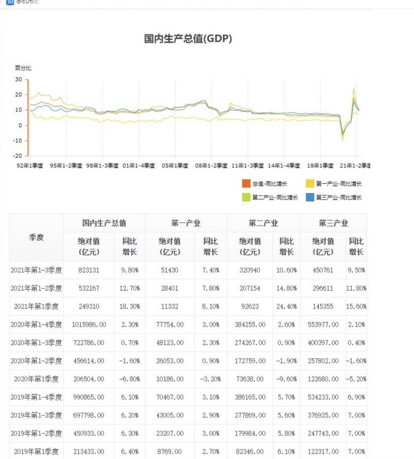
Gross domestic product (GDP) refers to the final result of the production activities of all resident units of a country (or region) in a certain period calculated according to the national market price. It is often recognized as the best indicator to measure the national economic situation. GDP is an important comprehensive statistical index in the accounting system; It is also the core index in China's new national economic accounting system. It reflects the economic strength and market scale of a country (or region). In recent years, with the rapid development of China's economy, GDP has also increased significantly. I want to analyze China's GDP in recent years through this climb.
(2) Theme web crawler design scheme
1. Topic crawler name
Climbing of domestic GDP
2. Content and data feature analysis of topic web crawler
The data value and year-on-year growth of the website's GDP and primary, secondary and tertiary industries.
3. Overview of thematic web crawler design scheme
Crawl the gdp data of the website, find the relevant data of the corresponding tag link, and then clean and visually analyze the data.
(3) Analysis of structural characteristics of theme pages
1. Structure and feature analysis of theme page
Crawl main page
In recent years, the GDP of each quarter, the production value of the primary, secondary and tertiary industries and their respective year-on-year growth ratios
2. HTML page parsing
3. Node (label) search method and traversal method
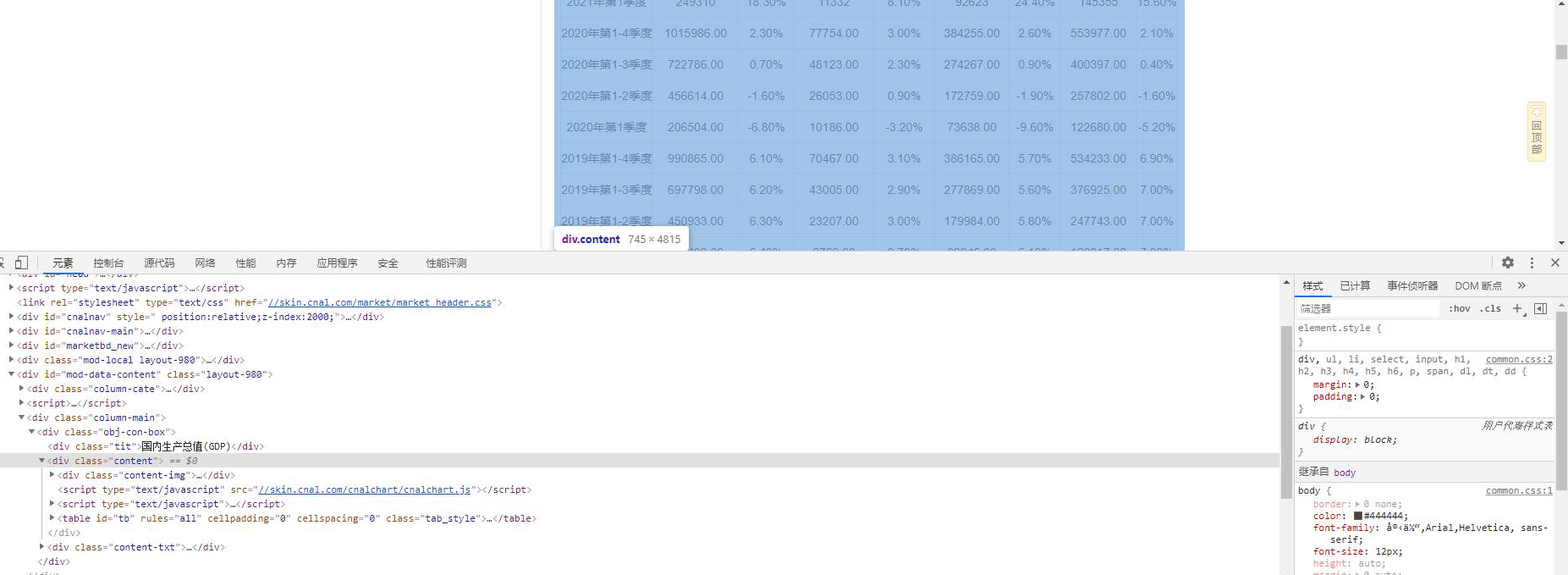
Review the elements of the website, and then find the data page under div class under the corresponding body tag.
(4) Web crawler program design
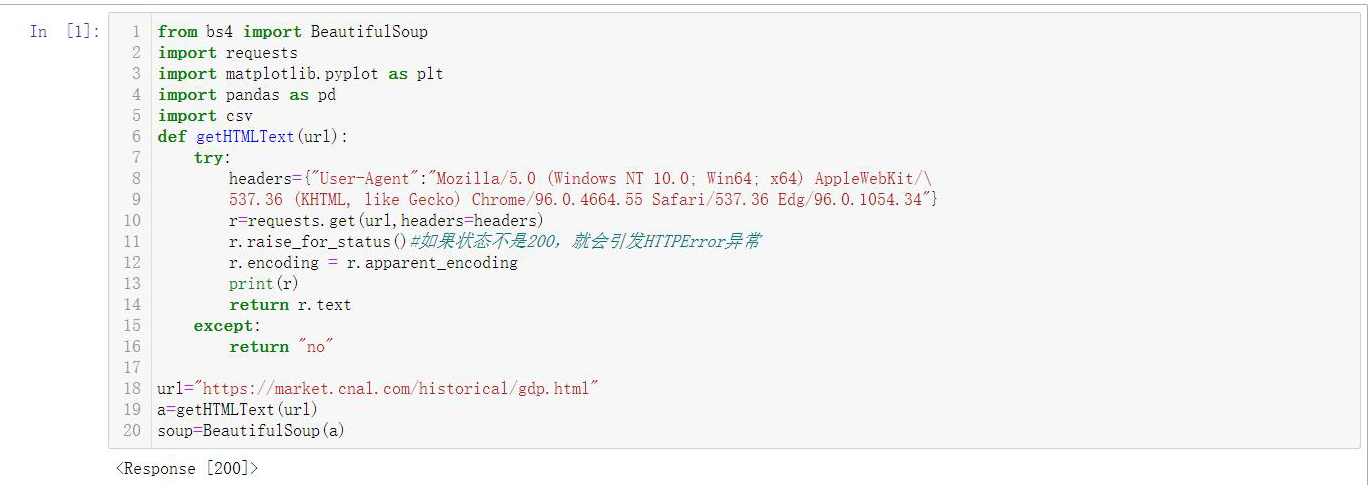
1. Data crawling and acquisition
 1 from bs4 import BeautifulSoup
 2 import requests
 3 import matplotlib.pyplot as plt
 4 import pandas as pd
 5 import csv
 6 def getHTMLText(url):
 7     try:
 8         headers={"User-Agent":"Mozilla/5.0 (Windows NT 10.0; Win64; x64) AppleWebKit/\
 9         537.36 (KHTML, like Gecko) Chrome/96.0.4664.55 Safari/537.36 Edg/96.0.1054.34"}
10         r=requests.get(url,headers=headers)
11         r.raise_for_status()#If the status is not 200, the HTTPError abnormal
12         r.encoding = r.apparent_encoding
13         print(r)
14         return r.text
15     except:
16         return "no"
17
18 url="https://market.cnal.com/historical/gdp.html"
19 a=getHTMLText(url)
20 soup=BeautifulSoup(a)
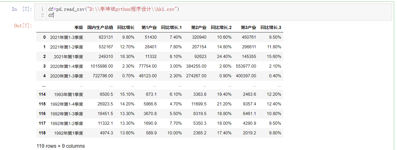
2. Clean and process the data
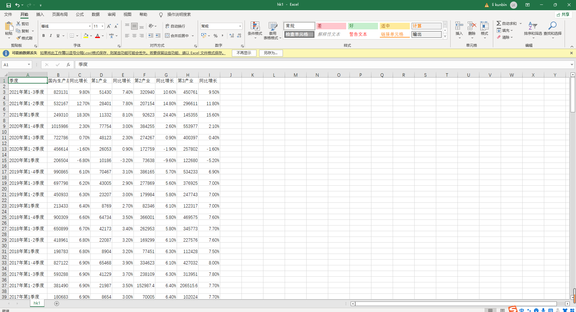
 1 fff=[]
 2
 3 for i in soup.find_all("tr")[2:]:
 4     fd=[]
 5     gg=0
 6     for a in i:
 7         if gg==1:
 8             fd.append(a)
 9         elif gg==3:
10             fd.append(a)
11         elif gg==5:
12             fd.append(a)
13         elif gg==7:
14             fd.append(a)
15         elif gg==9:
16             fd.append(a)
17         elif gg==11:
18             fd.append(a)
19         elif gg==13:
20             fd.append(a)
21         elif gg==15:
22             fd.append(a)
23         elif gg==17:
24             fd.append(a)
25         gg=gg+1
26     fff.append(fd)ght=[]
27 for gtk in fff:
28     hv=[]
29     for i in gtk:
30         hv.append(str(i)[4:-5])
31     ght.append(hv)with open("D:\\Li kunbin python Programming\\hk1.csv","w",encoding="utf_8_sig") as fi:
32     writer=csv.writer(fi)
33     writer.writerow(["quarter",
34                      "gross domestic product",
35                      "Year on year growth",
36                      "Primary industry",
37                      "Year on year growth",
38                      "Secondary industry",
39                      "Year on year growth",
40                      "Tertiary industry",
41                      "Year on year growth"])#Data column name for each column
42     for da in ght:
43         writer.writerow(da)
44 fi.close()
45 df=pd.read_csv("D:\\Li kunbin python Programming\\hk1.csv")
46 df
3 data analysis and visualization
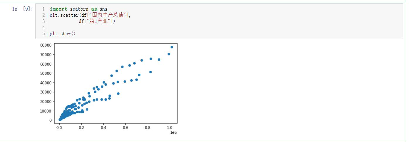
 1 for hji in range(len(df["quarter"])):
 2     df.loc[hji,"gross domestic product"]=float("".join(str(df.loc[hji,"gross domestic product"]).split(",")))
 3     df.loc[hji,"Primary industry"]=float("".join(str(df.loc[hji,"Primary industry"]).split(",")))
 4     df.loc[hji,"Secondary industry"]=float("".join(str(df.loc[hji,"Secondary industry"]).split(",")))
 5     df.loc[hji,"Tertiary industry"]=float("".join(str(df.loc[hji,"Tertiary industry"]).split(",")))
 6     df.loc[hji,"Year on year growth"]=float(str(df.loc[hji,"Year on year growth"])[0:-2])/100
 7     df.loc[hji,"Year on year growth.1"]=float(str(df.loc[hji,"Year on year growth.1"])[0:-2])/100
 8     df.loc[hji,"Year on year growth.2"]=float(str(df.loc[hji,"Year on year growth.2"])[0:-2])/100
 9     df.loc[hji,"Year on year growth.3"]=float(str(df.loc[hji,"Year on year growth.3"])[0:-2])/100import seaborn as sns
10 plt.scatter(df["gross domestic product"],
11            df["Primary industry"])
12
13 plt.show()
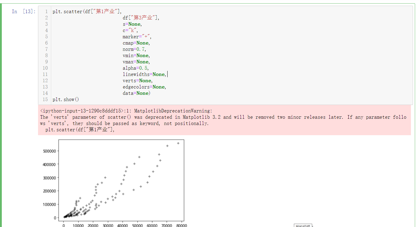
 1 plt.scatter(df["Primary industry"],
 2                           df["Tertiary industry"],
 3                           s=None,
 4                           c="k",
 5                           marker="+",
 6                           cmap=None,
 7                           norm=0.7,
 8                           vmin=None,
 9                           vmax=None,
10                           alpha=0.5,
11                           linewidths=None,
12                           verts=None,
13                           edgecolors=None,
14                           data=None)
15 plt.show()
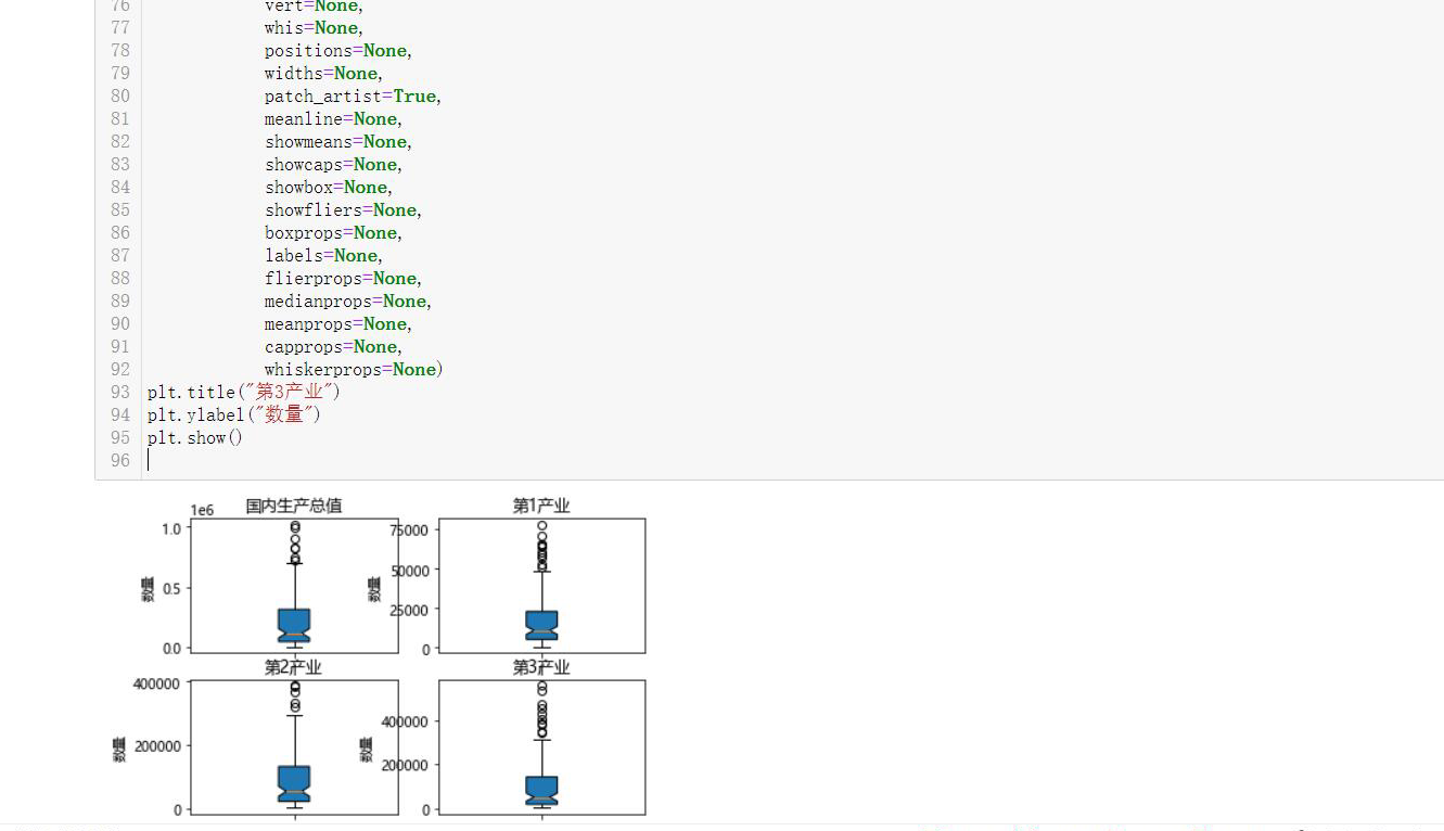
 1 #Understand the position and quantity distribution of the average production value through the box diagram
 2 plt.subplot(2,2,1)
 3 plt.boxplot(df["gross domestic product"],
 4             notch=True,
 5             sym=None,
 6             vert=None,
 7             whis=None,
 8             positions=None,
 9             widths=None,
10             patch_artist=True,
11             meanline=None,
12             showmeans=None,
13             showcaps=None,
14             showbox=None,
15             showfliers=None,
16             boxprops=None,
17             labels=None,
18             flierprops=None,
19             medianprops=None,
20             meanprops=None,
21             capprops=None,
22             whiskerprops=None)
23 plt.title("gross domestic product")
24 plt.ylabel("quantity")
25 plt.subplot(2,2,2)
26 plt.boxplot(df["Primary industry"],
27             notch=True,
28             sym=None,
29             vert=None,
30             whis=None,
31             positions=None,
32             widths=None,
33             patch_artist=True,
34             meanline=None,
35             showmeans=None,
36             showcaps=None,
37             showbox=None,
38             showfliers=None,
39             boxprops=None,
40             labels=None,
41             flierprops=None,
42             medianprops=None,
43             meanprops=None,
44             capprops=None,
45             whiskerprops=None)
46 plt.title("Primary industry")
47 plt.ylabel("quantity")
48 plt.subplot(2,2,3)
49
50 plt.boxplot(df["Secondary industry"],
51             notch=True,
52             sym=None,
53             vert=None,
54             whis=None,
55             positions=None,
56             widths=None,
57             patch_artist=True,
58             meanline=None,
59             showmeans=None,
60             showcaps=None,
61             showbox=None,
62             showfliers=None,
63             boxprops=None,
64             labels=None,
65             flierprops=None,
66             medianprops=None,
67             meanprops=None,
68             capprops=None,
69             whiskerprops=None)
70 plt.title("Secondary industry")
71 plt.ylabel("quantity")
72 plt.subplot(2,2,4)
73 plt.boxplot(df["Tertiary industry"],
74             notch=True,
75             sym=None,
76             vert=None,
77             whis=None,
78             positions=None,
79             widths=None,
80             patch_artist=True,
81             meanline=None,
82             showmeans=None,
83             showcaps=None,
84             showbox=None,
85             showfliers=None,
86             boxprops=None,
87             labels=None,
88             flierprops=None,
89             medianprops=None,
90             meanprops=None,
91             capprops=None,
92             whiskerprops=None)
93 plt.title("Tertiary industry")
94 plt.ylabel("quantity")
95 plt.show()
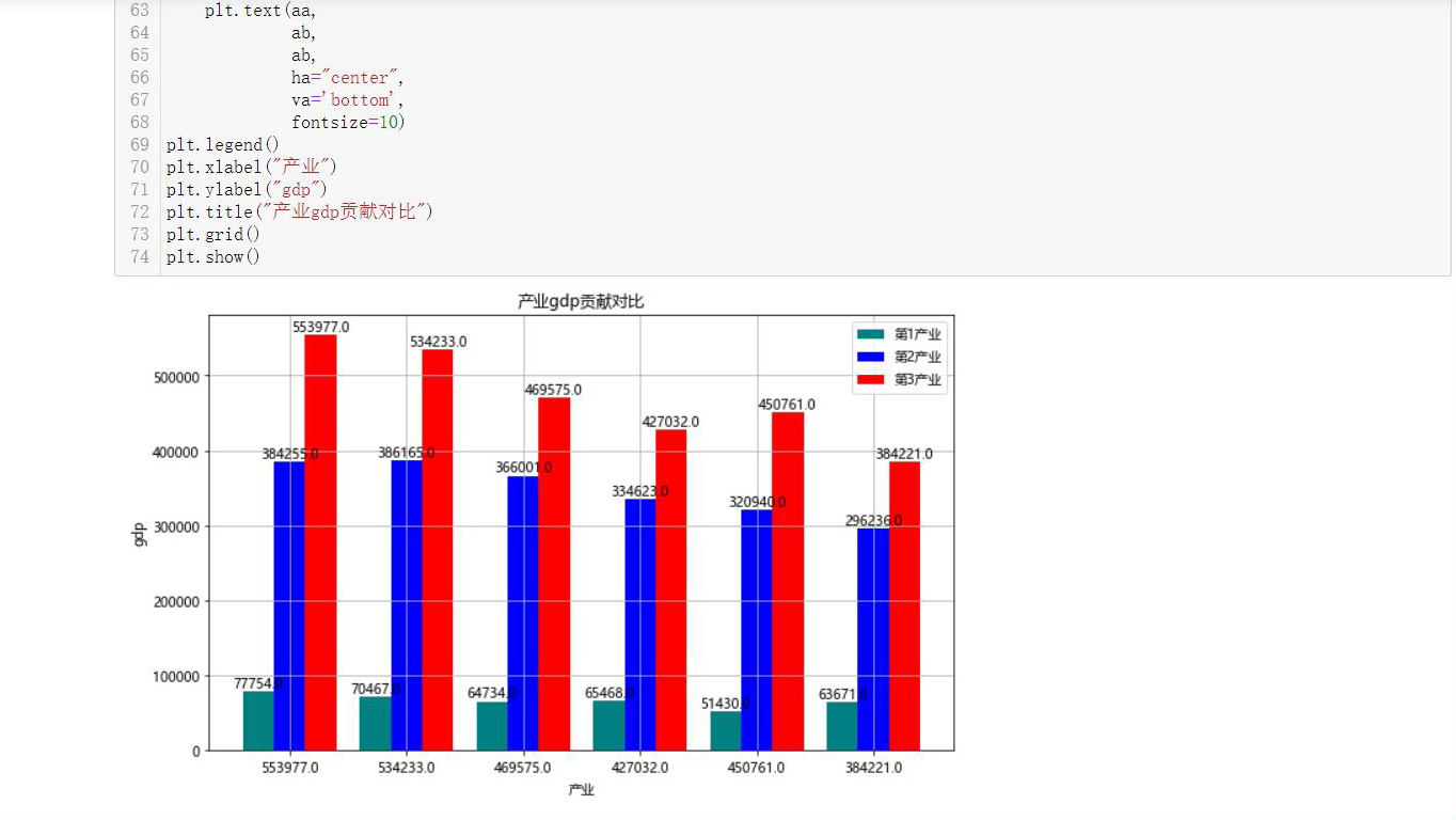
 1 import requests
 2 from bs4 import BeautifulSoup
 3 import matplotlib.pyplot as plt
 4 import seaborn as sns
 5 import pandas as pd
 6 #df=pd.read_csv("C:\\Users\\wei\\data.csv")
 7 ggf=df.sort_values(by="gross domestic product",
 8                         axis=0,
 9                         ascending=False,)
10 bk=ggf["Primary industry"][0:6]
11 zk=ggf["Secondary industry"][0:6]
12 city_1=ggf["Tertiary industry"][0:6]
13 #Show Chinese labels,Dealing with Chinese garbled code
14 plt.rcParams['font.sans-serif']=['Microsoft YaHei']
15 plt.rcParams['axes.unicode_minus']=False
16 plt.figure(figsize=(10,6))
17 x=list(range(len(zk)))
18 #Set spacing for pictures
19 total_width=0.8
20 n=3
21 width=total_width/n
22 for i in range(len(x)):
23     x[i]-=width
24 plt.bar(x,
25         bk,
26         width=width,
27         label="Primary industry",
28         fc="teal"
29        )
30 for aa,ab in zip(x,bk):
31     plt.text(aa,
32              ab,
33              ab,
34              ha="center",
35              va='bottom',
36              fontsize=10)
37 for i in range(len(x)):
38     x[i]+=width
39 plt.bar(x,
40         zk,
41         width=width,#width
42         label="Secondary industry",
43         tick_label=city_1,
44         color="b"
45        )
46 for aa,ab in zip(x,zk):
47     plt.text(aa,
48              ab,
49              ab,
50              ha="center",
51              va='bottom',
52              fontsize=10)
53
54 for i in range(len(x)):
55     x[i]+=width
56 plt.bar(x,
57         city_1,
58         width=width,
59         label="Tertiary industry",
60         color="r"
61        )
62 for aa,ab in zip(x,city_1):
63     plt.text(aa,
64              ab,
65              ab,
66              ha="center",
67              va='bottom',
68              fontsize=10)
69 plt.legend()
70 plt.xlabel("industry")
71 plt.ylabel("gdp")
72 plt.title("industry gdp Contribution comparison")
73 plt.grid()
74 plt.show()
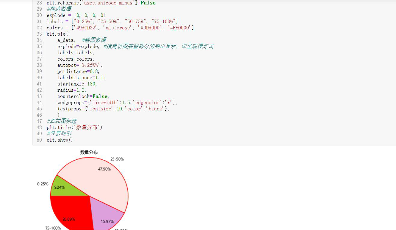
 1 #Organize drawing data
 2 hi=df.sort_values(by="gross domestic product",
 3                         axis=0,
 4                         ascending=False,)
 5 for ikl in range(len(df["gross domestic product"])):
 6     if ikl==29:
 7         fa=hi.loc[ikl,"gross domestic product"]
 8     elif ikl==60:
 9         fb=hi.loc[ikl,"gross domestic product"]
10     elif ikl==90:
11         fc=hi.loc[ikl,"gross domestic product"]
12 a_25=0
13 a_50=0
14 a_75=0
15 a_100=0
16 DF=len(hi["gross domestic product"])
17 for gh in range(DF):
18     if hi.loc[gh,"gross domestic product"]>fa:
19         a_100=a_100+1
20     elif hi.loc[gh,"gross domestic product"]>fb:
21         a_75=a_75+1
22     elif hi.loc[gh,"gross domestic product"]>fc:
23         a_50=a_50+1
24     else:
25         a_25=a_25+1
26 a_data=[a_25,a_50,a_75,a_100]
27 plt.rcParams['font.sans-serif']=['Microsoft YaHei']  #Show Chinese labels,Dealing with Chinese garbled code
28 plt.rcParams['axes.unicode_minus']=False
29 #Construction data
30 explode = [0, 0, 0, 0]
31 labels = ["0-25%", "25-50%", "50-75%", "75-100%"]
32 colors = ['#9ACD32', 'mistyrose', '#DDA0DD', '#FF0000']
33 plt.pie(
34     a_data,  #Drawing data
35     explode=explode, #Specifies that some parts of the pie chart are highlighted, that is, they appear explosive
36     labels=labels,
37     colors=colors,
38     autopct='%.2f%%',
39     pctdistance=0.8,
40     labeldistance=1.1,
41     startangle=180,
42     radius=1.2,
43     counterclock=False,
44     wedgeprops={'linewidth':1.5,'edgecolor':'r'},
45     textprops={'fontsize':10,'color':'black'},
46     )
47 #Add diagram title
48 plt.title('Quantity distribution')
49 #display graphics
50 plt.show()
4.4 data persistence
5. Summarize the codes of the above parts and attach the complete program code
  1 from bs4 import BeautifulSoup
  2 import requests
  3 import matplotlib.pyplot as plt
  4 import pandas as pd
  5 import csv
  6 def getHTMLText(url):
  7     try:
  8         headers={"User-Agent":"Mozilla/5.0 (Windows NT 10.0; Win64; x64) AppleWebKit/\
  9         537.36 (KHTML, like Gecko) Chrome/96.0.4664.55 Safari/537.36 Edg/96.0.1054.34"}
 10         r=requests.get(url,headers=headers)
 11         r.raise_for_status()#If the status is not 200, the HTTPError abnormal
 12         r.encoding = r.apparent_encoding
 13         print(r)
 14         return r.text
 15     except:
 16         return "no"
 17
 18 url="https://market.cnal.com/historical/gdp.html"
 19 a=getHTMLText(url)
 20 soup=BeautifulSoup(a)fff=[]
 21
 22 for i in soup.find_all("tr")[2:]:
 23     fd=[]
 24     gg=0
 25     for a in i:
 26         if gg==1:
 27             fd.append(a)
 28         elif gg==3:
 29             fd.append(a)
 30         elif gg==5:
 31             fd.append(a)
 32         elif gg==7:
 33             fd.append(a)
 34         elif gg==9:
 35             fd.append(a)
 36         elif gg==11:
 37             fd.append(a)
 38         elif gg==13:
 39             fd.append(a)
 40         elif gg==15:
 41             fd.append(a)
 42         elif gg==17:
 43             fd.append(a)
 44         gg=gg+1
 45     fff.append(fd)ght=[]
 46 for gtk in fff:
 47     hv=[]
 48     for i in gtk:
 49         hv.append(str(i)[4:-5])
 50     ght.append(hv)
 51 with open("D:\\Li kunbin python Programming\\hk1.csv","w",encoding="utf_8_sig") as fi:
 52     writer=csv.writer(fi)
 53     writer.writerow(["quarter",
 54                      "gross domestic product",
 55                      "Year on year growth",
 56                      "Primary industry",
 57                      "Year on year growth",
 58                      "Secondary industry",
 59                      "Year on year growth",
 60                      "Tertiary industry",
 61                      "Year on year growth"])#Data column name for each column
 62     for da in ght:
 63         writer.writerow(da)
 64 fi.close()
 65 df=pd.read_csv("D:\\Li kunbin python Programming\\hk1.csv")
 66 df
 67 for hji in range(len(df["quarter"])):
 68     df.loc[hji,"gross domestic product"]=float("".join(str(df.loc[hji,"gross domestic product"]).split(",")))
 69     df.loc[hji,"Primary industry"]=float("".join(str(df.loc[hji,"Primary industry"]).split(",")))
 70     df.loc[hji,"Secondary industry"]=float("".join(str(df.loc[hji,"Secondary industry"]).split(",")))
 71     df.loc[hji,"Tertiary industry"]=float("".join(str(df.loc[hji,"Tertiary industry"]).split(",")))
 72     df.loc[hji,"Year on year growth"]=float(str(df.loc[hji,"Year on year growth"])[0:-2])/100
 73     df.loc[hji,"Year on year growth.1"]=float(str(df.loc[hji,"Year on year growth.1"])[0:-2])/100
 74     df.loc[hji,"Year on year growth.2"]=float(str(df.loc[hji,"Year on year growth.2"])[0:-2])/100
 75     df.loc[hji,"Year on year growth.3"]=float(str(df.loc[hji,"Year on year growth.3"])[0:-2])/100
 76 mport seaborn as sns
 77 plt.scatter(df["gross domestic product"],
 78            df["Primary industry"])
 79
 80 plt.show()
 81 plt.scatter(df["Primary industry"],
 82                           df["Tertiary industry"],
 83                           s=None,
 84                           c="k",
 85                           marker="+",
 86                           cmap=None,
 87                           norm=0.7,
 88                           vmin=None,
 89                           vmax=None,
 90                           alpha=0.5,
 91                           linewidths=None,
 92                           verts=None,
 93                           edgecolors=None,
 94                           data=None)
 95 plt.show()
 96 #Understand the position and quantity distribution of the average production value through the box diagram
 97 plt.subplot(2,2,1)
 98 plt.boxplot(df["gross domestic product"],
 99             notch=True,
100             sym=None,
101             vert=None,
102             whis=None,
103             positions=None,
104             widths=None,
105             patch_artist=True,
106             meanline=None,
107             showmeans=None,
108             showcaps=None,
109             showbox=None,
110             showfliers=None,
111             boxprops=None,
112             labels=None,
113             flierprops=None,
114             medianprops=None,
115             meanprops=None,
116             capprops=None,
117             whiskerprops=None)
118 plt.title("gross domestic product")
119 plt.ylabel("quantity")
120 plt.subplot(2,2,2)
121 plt.boxplot(df["Primary industry"],
122             notch=True,
123             sym=None,
124             vert=None,
125             whis=None,
126             positions=None,
127             widths=None,
128             patch_artist=True,
129             meanline=None,
130             showmeans=None,
131             showcaps=None,
132             showbox=None,
133             showfliers=None,
134             boxprops=None,
135             labels=None,
136             flierprops=None,
137             medianprops=None,
138             meanprops=None,
139             capprops=None,
140             whiskerprops=None)
141 plt.title("Primary industry")
142 plt.ylabel("quantity")
143 plt.subplot(2,2,3)
144
145 plt.boxplot(df["Secondary industry"],
146             notch=True,
147             sym=None,
148             vert=None,
149             whis=None,
150             positions=None,
151             widths=None,
152             patch_artist=True,
153             meanline=None,
154             showmeans=None,
155             showcaps=None,
156             showbox=None,
157             showfliers=None,
158             boxprops=None,
159             labels=None,
160             flierprops=None,
161             medianprops=None,
162             meanprops=None,
163             capprops=None,
164             whiskerprops=None)
165 plt.title("Secondary industry")
166 plt.ylabel("quantity")
167 plt.subplot(2,2,4)
168 plt.boxplot(df["Tertiary industry"],
169             notch=True,
170             sym=None,
171             vert=None,
172             whis=None,
173             positions=None,
174             widths=None,
175             patch_artist=True,
176             meanline=None,
177             showmeans=None,
178             showcaps=None,
179             showbox=None,
180             showfliers=None,
181             boxprops=None,
182             labels=None,
183             flierprops=None,
184             medianprops=None,
185             meanprops=None,
186             capprops=None,
187             whiskerprops=None)
188 plt.title("Tertiary industry")
189 plt.ylabel("quantity")
190 plt.show()
191 #Organize drawing data
192 hi=df.sort_values(by="gross domestic product",
193                         axis=0,
194                         ascending=False,)
195 for ikl in range(len(df["gross domestic product"])):
196     if ikl==29:
197         fa=hi.loc[ikl,"gross domestic product"]
198     elif ikl==60:
199         fb=hi.loc[ikl,"gross domestic product"]
200     elif ikl==90:
201         fc=hi.loc[ikl,"gross domestic product"]
202 a_25=0
203 a_50=0
204 a_75=0
205 a_100=0
206 DF=len(hi["gross domestic product"])
207 for gh in range(DF):
208     if hi.loc[gh,"gross domestic product"]>fa:
209         a_100=a_100+1
210     elif hi.loc[gh,"gross domestic product"]>fb:
211         a_75=a_75+1
212     elif hi.loc[gh,"gross domestic product"]>fc:
213         a_50=a_50+1
214     else:
215         a_25=a_25+1
216 a_data=[a_25,a_50,a_75,a_100]
217 plt.rcParams['font.sans-serif']=['Microsoft YaHei']  #Show Chinese labels,Dealing with Chinese garbled code
218 plt.rcParams['axes.unicode_minus']=False
219 #Construction data
220 explode = [0, 0, 0, 0]
221 labels = ["0-25%", "25-50%", "50-75%", "75-100%"]
222 colors = ['#9ACD32', 'mistyrose', '#DDA0DD', '#FF0000']
223 plt.pie(
224     a_data,  #Drawing data
225     explode=explode, #Specifies that some parts of the pie chart are highlighted, that is, they appear explosive
226     labels=labels,
227     colors=colors,
228     autopct='%.2f%%',
229     pctdistance=0.8,
230     labeldistance=1.1,
231     startangle=180,
232     radius=1.2,
233     counterclock=False,
234     wedgeprops={'linewidth':1.5,'edgecolor':'r'},
235     textprops={'fontsize':10,'color':'black'},
236     )
237 #Add diagram title
238 plt.title('Quantity distribution')
239 #display graphics
240 plt.show()
241 import requests
242 from bs4 import BeautifulSoup
243 import matplotlib.pyplot as plt
244 import seaborn as sns
245 import pandas as pd
246 #df=pd.read_csv("C:\\Users\\wei\\data.csv")
247 ggf=df.sort_values(by="gross domestic product",
248                         axis=0,
249                         ascending=False,)
250 bk=ggf["Primary industry"][0:6]
251 zk=ggf["Secondary industry"][0:6]
252 city_1=ggf["Tertiary industry"][0:6]
253 #Show Chinese labels,Dealing with Chinese garbled code
254 plt.rcParams['font.sans-serif']=['Microsoft YaHei']
255 plt.rcParams['axes.unicode_minus']=False
256 plt.figure(figsize=(10,6))
257 x=list(range(len(zk)))
258 #Set spacing for pictures
259 total_width=0.8
260 n=3
261 width=total_width/n
262 for i in range(len(x)):
263     x[i]-=width
264 plt.bar(x,
265         bk,
266         width=width,
267         label="Primary industry",
268         fc="teal"
269        )
270 for aa,ab in zip(x,bk):
271     plt.text(aa,
272              ab,
273              ab,
274              ha="center",
275              va='bottom',
276              fontsize=10)
277 for i in range(len(x)):
278     x[i]+=width
279 plt.bar(x,
280         zk,
281         width=width,#width
282         label="Secondary industry",
283         tick_label=city_1,
284         color="b"
285        )
286 for aa,ab in zip(x,zk):
287     plt.text(aa,
288              ab,
289              ab,
290              ha="center",
291              va='bottom',
292              fontsize=10)
293
294 for i in range(len(x)):
295     x[i]+=width
296 plt.bar(x,
297         city_1,
298         width=width,
299         label="Tertiary industry",
300         color="r"
301        )
302 for aa,ab in zip(x,city_1):
303     plt.text(aa,
304              ab,
305              ab,
306              ha="center",
307              va='bottom',
308              fontsize=10)
309 plt.legend()
310 plt.xlabel("industry")
311 plt.ylabel("gdp")
312 plt.title("industry gdp Contribution comparison")
313 plt.grid()
314 plt.show()
(5) . summary
1. What conclusions can be drawn from the analysis and visualization of subject data? Is the expected goal achieved?
Through this course design, I have a clear understanding of the growth and decline of China's GDP and the situation of their respective industries in recent years, and have a deeper understanding of China's economic situation.
2. What are the gains in the process of completing this design? And suggestions for improvement?
In this course, I have mastered deeper knowledge of crawlers and stimulated my interest in crawlers and python. Many difficulties were encountered in the design process,
Through online information search and online video teaching, I am very helpful in this course design,
In short, this design has benefited me a lot and made me understand that I still have a lot of knowledge to learn. I will continue to refuel and study hard.