catalogue
- Import data
- Missing and outlier handling
- Feature visualization
- feature selection
- model training
- Model evaluation
- Model result transfer score
- Calculate user total score
1, Import data
Reply to key words in official account python wind control model: learning materials
#Import module
import pandas as pd
import numpy as np
from scipy import stats
import seaborn as sns
import matplotlib.pyplot as plt
%matplotlib inline
plt.rc("font",family="SimHei",size="12")  #Solve the problem that Chinese cannot be displayed

#Import data
train=pd.read_csv('F:\\python\\Give-me-some-credit-master\\data\\cs-training.csv')
Simple view of data information
#Simple view data
train.info()

'''
train.info()
<class 'pandas.core.frame.DataFrame'>
RangeIndex: 150000 entries, 0 to 149999
Data columns (total 12 columns):
Unnamed: 0                              150000 non-null int64
SeriousDlqin2yrs                        150000 non-null int64
RevolvingUtilizationOfUnsecuredLines    150000 non-null float64
age                                     150000 non-null int64
NumberOfTime30-59DaysPastDueNotWorse    150000 non-null int64
DebtRatio                               150000 non-null float64
MonthlyIncome                           120269 non-null float64
NumberOfOpenCreditLinesAndLoans         150000 non-null int64
NumberOfTimes90DaysLate                 150000 non-null int64
NumberRealEstateLoansOrLines            150000 non-null int64
NumberOfTime60-89DaysPastDueNotWorse    150000 non-null int64
NumberOfDependents                      146076 non-null float64
dtypes: float64(4), int64(8)
memory usage: 13.7 MB

'''
Data viewing of the first three rows and the last three rows
#Data viewing of the first three rows and the last three rows
train.head(3).append(train.tail(3))
shape view
#shape
train.shape  #(150000, 11)
Convert English fields to Chinese field names for easy understanding
states={'Unnamed: 0':'id',
        'SeriousDlqin2yrs':'Good and bad customers',
        'RevolvingUtilizationOfUnsecuredLines':'Available limit ratio',
        'age':'Age',
        'NumberOfTime30-59DaysPastDueNotWorse':'Overdue 30-59 Tianbi number',
        'DebtRatio':'Debt ratio',
        'MonthlyIncome':'monthly income',
        'NumberOfOpenCreditLinesAndLoans':'Credit quantity',
        'NumberOfTimes90DaysLate':'Number of transactions overdue for 90 days',
        'NumberRealEstateLoansOrLines':'Fixed asset loans',
        'NumberOfTime60-89DaysPastDueNotWorse':'Overdue 60-89 Tianbi number',
        'NumberOfDependents':'Number of family members'}
train.rename(columns=states,inplace=True)

#catalog index
train=train.set_index('id',drop=True)
descriptive statistics

2, Missing and outlier handling
1. Missing value processing
View missing values
#Check the missing condition of each column
train.isnull().sum()
#Check the missing proportion
train.isnull().sum()/len(train)
#Missing value visualization
missing=train.isnull().sum()
missing[missing>0].sort_values().plot.bar()  #Take out and sort those greater than 0
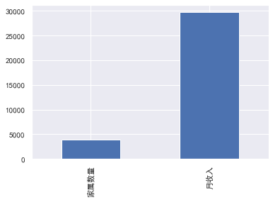
knowable
The missing value of monthly income is 29731, and the missing proportion is 0.198207
Missing value of number of family members: 3924, missing ratio: 0.026160
First copy a copy of data, retain the original data, and then process the missing values
#Keep original data
train_cp=train.copy()

#Monthly income uses the average to fill in the missing value
train_cp.fillna({'monthly income':train_cp['monthly income'].mean()},inplace=True)
train_cp.isnull().sum()

#Lines with missing number of family members are removed
train_cp=train_cp.dropna()
train_cp.shape   #(146076, 11)
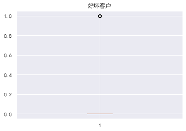
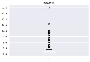
2. Abnormal value handling
View outliers
#View outliers
#Draw box diagram
for col in train_cp.columns:
    plt.boxplot(train_cp[col])
    plt.title(col)
    plt.show()

Data with an available quota ratio greater than 1 is abnormal
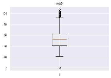
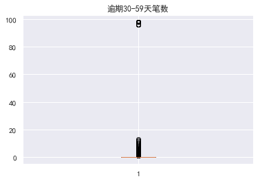
The data with an age of 0 is also abnormal. In fact, those younger than 18 can be identified as abnormal. There is a super outlier data for those who are 30-59 days overdue
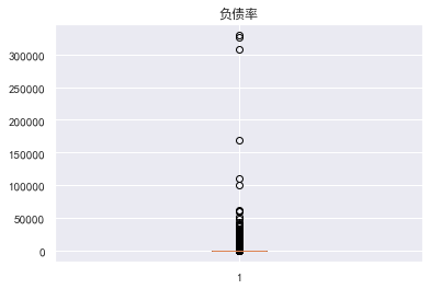


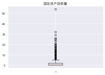

Outlier processing eliminates illogical data and super outlier data. The ratio of available quota should be less than 1. Outliers with age of 0 and super outlier data with overdue days of more than 80 are filtered out to filter out the remaining data
train_cp=train_cp[train_cp['Available limit ratio']<1]
train_cp=train_cp[train_cp['Age']>0]
train_cp=train_cp[train_cp['Overdue 30-59 Tianbi number']<80]
train_cp=train_cp[train_cp['Overdue 60-89 Tianbi number']<80]
train_cp=train_cp[train_cp['Number of transactions overdue for 90 days']<80]
train_cp=train_cp[train_cp['Fixed asset loans']<50]
train_cp=train_cp[train_cp['Debt ratio']<5000]
train_cp.shape  #(141180, 11)
3, Feature visualization
1. Univariate visualization
Good and bad users
#Good and bad users train_cp.info() train_cp['Good and bad customers'].value_counts() train_cp['Good and bad customers'].value_counts()/len(train_cp) train_cp['Good and bad customers'].value_counts().plot.bar() ''' 0 132787 1 8393 Name: Good and bad customers, dtype: int64 The data is heavily skewed 0 0.940551 1 0.059449 Name: Good and bad customers, dtype: float64 ''' 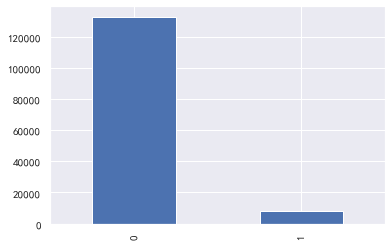 knowable y The value is heavily skewed **Available limit ratio and debt ratio**
#Available limit ratio and debt ratio
train_cp ['available quota ratio']. plot.hist()
train_cp ['debt ratio'. plot.hist()
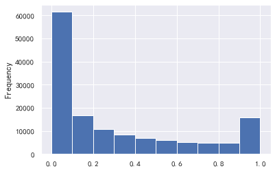
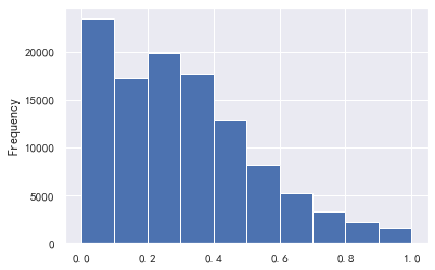
#The data with a debt ratio greater than 1 has too much impact
a=train_cp ['debt ratio']
a[a<=1].plot.hist()
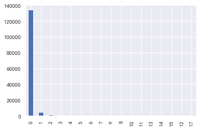
 ### 30-59 days overdue, 90 days overdue, 60-89 days overdue
#30-59 days overdue, 90 days overdue, 60-89 days overdue
for i,col in enumerate(['30-59 days overdue', '90 days overdue', '60-89 days overdue'):
plt.subplot(1,3,i+1)
train_cp[col].value_counts().plot.bar()
plt.title(col)
train_cp ['number of overdue transactions 30-59 days']. value_counts().plot.bar()
train_cp ['number of transactions overdue for 90 days']. value_counts().plot.bar()
train_cp ['number of overdue transactions 60-89 days']. value_counts().plot.bar()
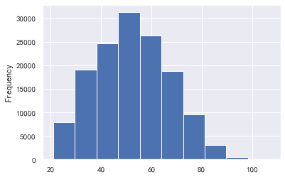
   ### Age: basically in line with normal distribution
#Age
train_cp ['age'. plot.hist()
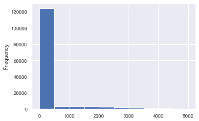
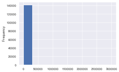
 ### monthly income
#Monthly income
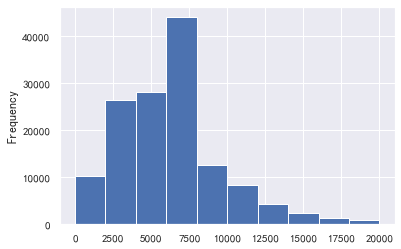
train_cp ['monthly income']. plot.hist()
sns.distplot(train_cp ['monthly income'])
#The influence of super outliers is too great. We take the data less than 5w to draw the graph
a=train_cp ['monthly income']
a[a<=50000].plot.hist()
#If it is found that there are not many less than 50000, take 2w
a=train_cp ['monthly income']
a[a<=20000].plot.hist()
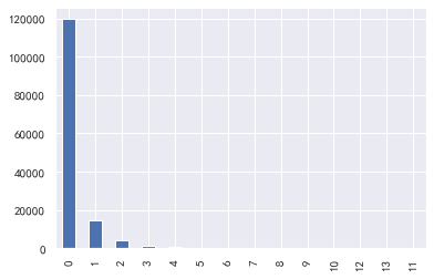
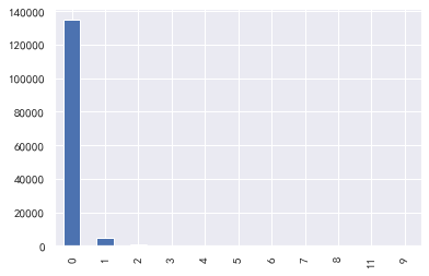
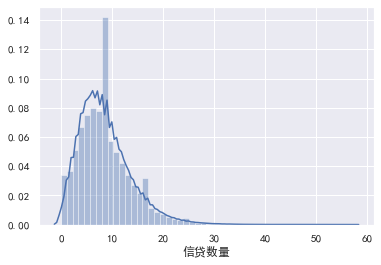
 ### Credit quantity
#Credit quantity
train_cp ['credit quantity']. value_counts().plot.bar()
sns.distplot(train_cp ['credit quantity'])
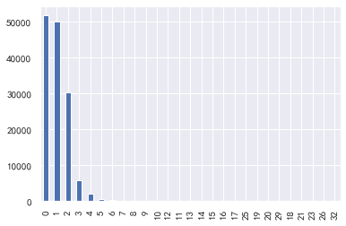
 ### Fixed asset loans
#Fixed asset loans
train_cp ['fixed asset loan volume']. value_counts().plot.bar()
sns.distplot(train_cp ['fixed asset loan volume'])
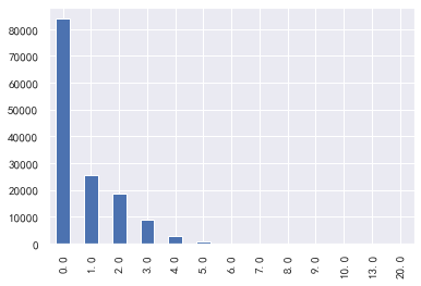
 ### Number of family members
#Number of family members
train_cp ['number of family members']. value_counts().plot.bar()
sns.distplot(train_cp ['number of family members'])
 2.Univariate and y Value visualization ----------- ### Available limit ratio
#Univariate and y-value visualization
#Available quota ratio, debt ratio, age and monthly income need to be separated
#Available limit ratio
train_ CP ['available quota ratio'] = pd.cut(train_cp ['available quota ratio'], 5)
pd.crosstab(train_cp ['available quota ratio _cut'], train_cp ['good and bad customers']. plot(kind = "bar")
a=pd.crosstab(train_cp ['available quota ratio _cut'], train_cp ['good and bad customers'])
A ['proportion of bad users'] = a[1]/(a[0]+a[1])
a ['proportion of bad users']. plot()
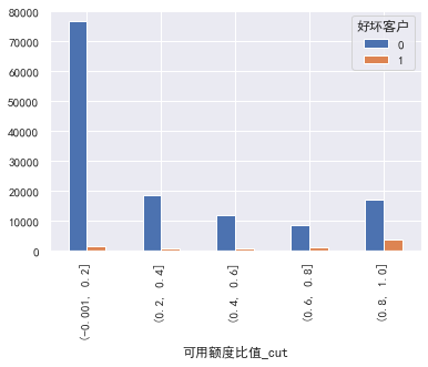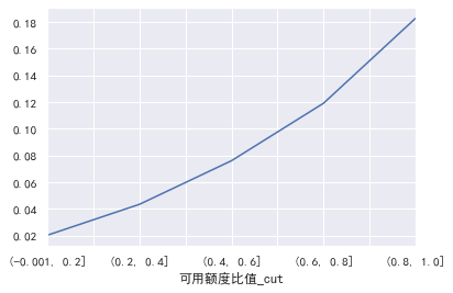 It can be seen that the overdue rate of each box at the end of the box division is only 6 times worse, indicating that this feature is still good ### Debt ratio
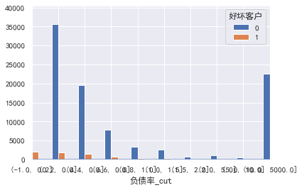
#Debt ratio
cut=[-1,0.2,0.4,0.6,0.8,1,1.5,2,5,10,5000]
train_ CP ['debt ratio'] = pd.cut(train_cp ['debt ratio'], bins=cut)
pd.crosstab(train_cp ['debt ratio _cut'], train_cp ['good and bad customers']. plot(kind = "bar")
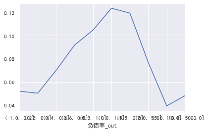
a=pd.crosstab(train_cp ['debt ratio _cut'], train_cp ['good and bad customers'])
A ['proportion of bad users'] = a[1]/(a[0]+a[1])
a ['proportion of bad users']. plot()
 ### Age
#Age
cut=[0,30,40,50,60,100]
train_ CP ['age _cut '] = pd.cut(train_cp ['age'], bins=cut)
pd.crosstab(train_cp ['age _cut'], train_cp ['good and bad customers']. plot(kind = "bar")
a=pd.crosstab(train_cp ['age _cut'], train_cp ['good and bad customers'])
A ['proportion of bad users'] = a[1]/(a[0]+a[1])
a ['proportion of bad users']. plot()
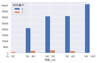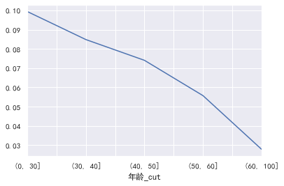 Why are there so many elderly people? It's unrealistic. Are the products mainly aimed at elderly users ### monthly income 
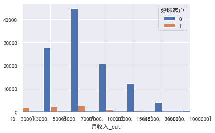
#Monthly income
cut=[0,3000,5000,7000,10000,15000,30000,1000000]
train_ CP ['monthly income _cut '] = pd.cut(train_cp ['monthly income'], bins=cut)
pd.crosstab(train_cp ['monthly revenue _cut'], train_cp ['good and bad customers']. plot(kind = "bar")
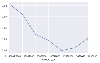
a=pd.crosstab(train_cp ['monthly revenue _cut'], train_cp ['good and bad customers'])
A ['proportion of bad users'] = a[1]/(a[0]+a[1])
a ['proportion of bad users']. plot()
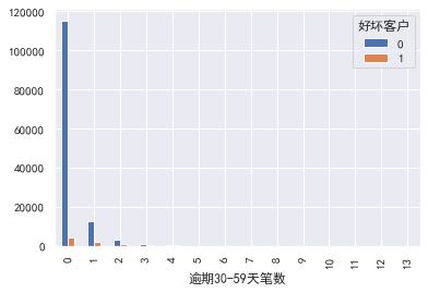
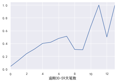
 Overdue 30-59 Tianbi number,Number of transactions overdue for 90 days,Overdue 60-89 Tianbi number \\Credit quantity\\Fixed asset loans\\The number of family members does not need to be divided into boxes for the time being: ### 30-59 days overdue
#30-59 days overdue, 90 days overdue, 60-89 days overdue \ amount of credit \ amount of fixed asset loans \ number of family members
#30-59 days overdue
pd.crosstab(train_cp ['30-59 days overdue], train_cp [' good and bad customers'). plot(kind = "bar")
a=pd.crosstab(train_cp ['30-59 days overdue], train_cp [' good and bad customers'])
A ['proportion of bad users'] = a[1]/(a[0]+a[1])
a ['proportion of bad users']. plot()
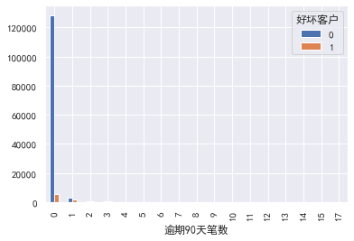
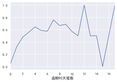
 ### Number of transactions overdue for 90 days
#Number of transactions overdue for 90 days
pd.crosstab(train_cp ['90 days overdue'], train_cp ['good and bad customers']. plot(kind = "bar")
a=pd.crosstab(train_cp ['90 days overdue], train_cp [' good and bad customers'])
A ['proportion of bad users'] = a[1]/(a[0]+a[1])
a ['proportion of bad users']. plot()
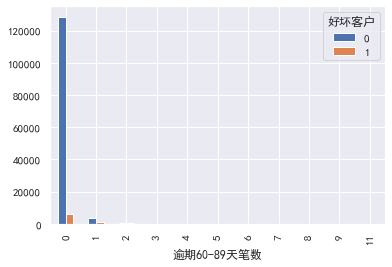
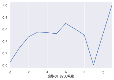
 ### 60-89 days overdue
#60-89 days overdue
pd.crosstab(train_cp ['60-89 days overdue'], train_cp ['good and bad customers']. plot(kind = "bar")
a=pd.crosstab(train_cp ['60-89 days overdue], train_cp [' good and bad customers'])
A ['proportion of bad users'] = a[1]/(a[0]+a[1])
a ['proportion of bad users']. plot()
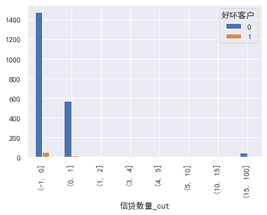
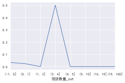
 ### Credit quantity 
#Credit quantity
cut=[-1,0,1,2,3,4,5,10,15,100]
train_ CP ['credit quantity _cut'] = pd.cut(train_cp ['monthly income'], bins=cut)
pd.crosstab(train_cp ['credit quantity _cut'], train_cp ['good and bad customers']. plot(kind = "bar")
a=pd.crosstab(train_cp ['credit quantity _cut'], train_cp ['good and bad customers'])
A ['proportion of bad users'] = a[1]/(a[0]+a[1])
a ['proportion of bad users']. plot()
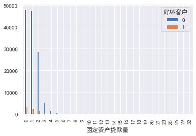
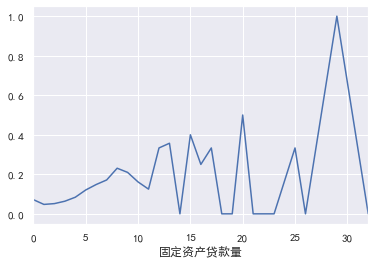
  ### Fixed asset loans
#Fixed asset loans
pd.crosstab(train_cp ['fixed asset loan volume'], train_cp ['good and bad customers']. plot(kind = "bar")
a=pd.crosstab(train_cp ['fixed asset loan volume'], train_cp ['good and bad customers'])
A ['proportion of bad users'] = a[1]/(a[0]+a[1])
a ['proportion of bad users']. plot()
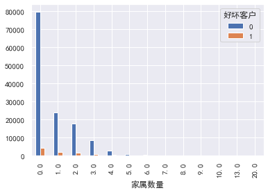
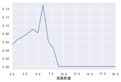
 ### Number of family members
#Number of family members
pd.crosstab(train_cp ['number of family members'], train_cp [' good and bad customers']. plot(kind = "bar")
a=pd.crosstab(train_cp ['number of family members'], train_cp [' good and bad customers'])
A ['proportion of bad users'] = a[1]/(a[0]+a[1])
a ['proportion of bad users']. plot()
 3.Correlation between variables: -----------
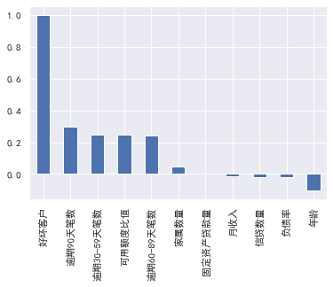
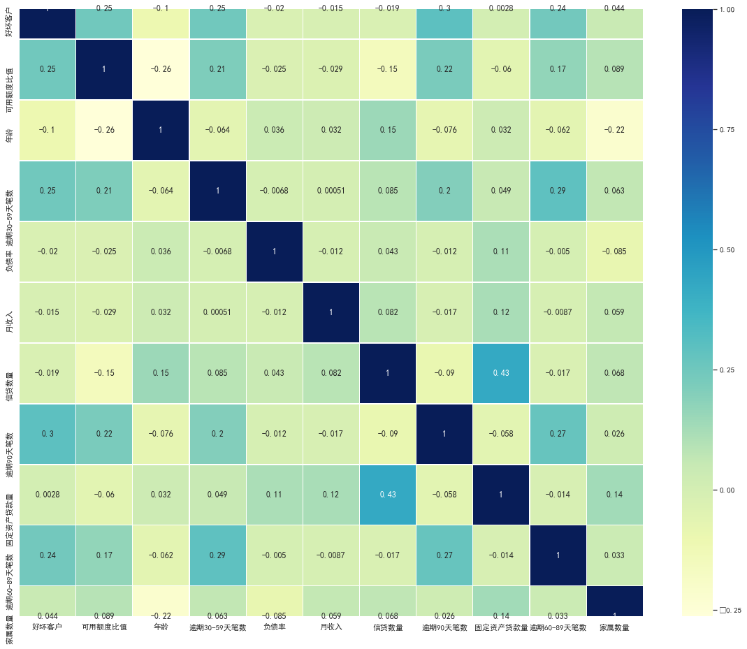
#Correlation between variables
train_cp.corr() ['good and bad customers']. sort_values(ascending = False).plot(kind=‘bar’)
plt.figure(figsize=(20,16))
corr=train_cp.corr()
sns.heatmap(corr, xticklabels=corr.columns, yticklabels=corr.columns,
linewidths=0.2, cmap="YlGnBu",annot=True)
  **4, Feature selection** ---------- 1.woe Sub box -------
#woe sub box
cut1=pd.qcut(train_cp ["available quota ratio"], 4,labels=False)
cut2=pd.qcut(train_cp ["age"], 8,labels=False)
bins3=[-1,0,1,3,5,13]
cut3=pd.cut(train_cp ["30-59 days overdue"], bins3,labels=False)
cut4=pd.qcut(train_cp ["debt ratio"], 3,labels=False)
cut5=pd.qcut(train_cp ["monthly income"], 4,labels=False)
cut6=pd.qcut(train_cp ["credit quantity"], 4,labels=False)
bins7=[-1, 0, 1, 3,5, 20]
cut7=pd.cut(train_cp ["90 days overdue"], bins7,labels=False)
bins8=[-1, 0,1,2, 3, 33]
cut8=pd.cut(train_cp ["fixed asset loan amount"], bins8,labels=False)
bins9=[-1, 0, 1, 3, 12]
cut9=pd.cut(train_cp ["60-89 days overdue"], bins9,labels=False)
bins10=[-1, 0, 1, 2, 3, 5, 21]
cut10=pd.cut(train_cp ["number of family members"], bins10,labels=False)
2. Calculation of woe value
The ratio of bad customers to good customers in the current group, and the difference between this ratio in all samples
#woe calculation
rate=train_cp["Good and bad customers"].sum()/(train_cp["Good and bad customers"].count()-train_cp["Good and bad customers"].sum())  #rate = bad / (total bad)
def get_woe_data(cut):
    grouped=train_cp["Good and bad customers"].groupby(cut,as_index = True).value_counts()
    woe=np.log(grouped.unstack().iloc[:,1]/grouped.unstack().iloc[:,0]/rate)
    return woe
cut1_woe=get_woe_data(cut1)
cut2_woe=get_woe_data(cut2)
cut3_woe=get_woe_data(cut3)
cut4_woe=get_woe_data(cut4)
cut5_woe=get_woe_data(cut5)
cut6_woe=get_woe_data(cut6)
cut7_woe=get_woe_data(cut7)
cut8_woe=get_woe_data(cut8)
cut9_woe=get_woe_data(cut9)
cut10_woe=get_woe_data(cut10)
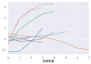
Visualize:
l=[cut1_woe,cut2_woe,cut3_woe,cut4_woe,cut5_woe,cut6_woe,cut7_woe,cut8_woe,cut9_woe,cut10_woe]
for i,col in enumerate(l):
    col.plot()
3.iv value calculation
iv value is actually equal to woe * (the proportion of bad customers in the current group to all bad customers - the proportion of good customers in the current group to all good customers)
#iv value calculation
def get_IV_data(cut,cut_woe):
    grouped=train_cp["Good and bad customers"].groupby(cut,as_index = True).value_counts()
    cut_IV=((grouped.unstack().iloc[:,1]/train_cp["Good and bad customers"].sum()-grouped.unstack().iloc[:,0]/(train_cp["Good and bad customers"].count()-train_cp["Good and bad customers"].sum()))*cut_woe).sum()
    return cut_IV
#Calculate the IV value of each group
cut1_IV=get_IV_data(cut1,cut1_woe)
cut2_IV=get_IV_data(cut2,cut2_woe)
cut3_IV=get_IV_data(cut3,cut3_woe)
cut4_IV=get_IV_data(cut4,cut4_woe)
cut5_IV=get_IV_data(cut5,cut5_woe)
cut6_IV=get_IV_data(cut6,cut6_woe)
cut7_IV=get_IV_data(cut7,cut7_woe)
cut8_IV=get_IV_data(cut8,cut8_woe)
cut9_IV=get_IV_data(cut9,cut9_woe)
cut10_IV=get_IV_data(cut10,cut10_woe)
IV=pd.DataFrame([cut1_IV,cut2_IV,cut3_IV,cut4_IV,cut5_IV,cut6_IV,cut7_IV,cut8_IV,cut9_IV,cut10_IV],index=['Available limit ratio','Age','Overdue 30-59 Tianbi number','Debt ratio','monthly income','Credit quantity','Number of transactions overdue for 90 days','Fixed asset loans','Overdue 60-89 Tianbi number','Number of family members'],columns=['IV'])
iv=IV.plot.bar(color='b',alpha=0.3,rot=30,figsize=(10,5),fontsize=(10))
iv.set_title('Characteristic variables and IV Value distribution diagram',fontsize=(15))
iv.set_xlabel('Characteristic variable',fontsize=(15))
iv.set_ylabel('IV',fontsize=(15))
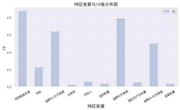

Generally, characteristic variables with IV greater than 0.02 are selected for follow-up training. It can be seen from the above that all variables meet the requirements, so all variables are selected
4.woe conversion
df_new=pd.DataFrame()   #New df_new stores the data converted by woe
def replace_data(cut,cut_woe):
    a=[]
    for i in cut.unique():
        a.append(i)
        a.sort()
    for m in range(len(a)):
        cut.replace(a[m],cut_woe.values[m],inplace=True)
    return cut
df_new["Good and bad customers"]=train_cp["Good and bad customers"]
df_new["Available limit ratio"]=replace_data(cut1,cut1_woe)
df_new["Age"]=replace_data(cut2,cut2_woe)
df_new["Overdue 30-59 Tianbi number"]=replace_data(cut3,cut3_woe)
df_new["Debt ratio"]=replace_data(cut4,cut4_woe)
df_new["monthly income"]=replace_data(cut5,cut5_woe)
df_new["Credit quantity"]=replace_data(cut6,cut6_woe)
df_new["Number of transactions overdue for 90 days"]=replace_data(cut7,cut7_woe)
df_new["Fixed asset loans"]=replace_data(cut8,cut8_woe)
df_new["Overdue 60-89 Tianbi number"]=replace_data(cut9,cut9_woe)
df_new["Number of family members"]=replace_data(cut10,cut10_woe)
df_new.head()
5, Model training
The main algorithm model used by credit scoring card is logistic regression. Logistic model is less sensitive to customer group changes than other high complexity models, so it is more robust and robust. In addition, the model is intuitive, the meaning of the coefficient is easy to explain and understand, and the advantage of using logical regression is that it can obtain the linear relationship between variables and the corresponding characteristic weight, which is convenient to convert it into one-to-one corresponding score form later
model training
#model training
from sklearn.linear_model import LogisticRegression
from sklearn.model_selection import train_test_split
x=df_new.iloc[:,1:]
y=df_new.iloc[:,:1]
x_train,x_test,y_train,y_test=train_test_split(x,y,test_size=0.6,random_state=0)
model=LogisticRegression()
clf=model.fit(x_train,y_train)
print('Test results:{}'.format(clf.score(x_test,y_test)))
Test score: 0.9427326816829579, which seems to be very high. In fact, it is caused by too serious data skew. The final result depends on auc
Calculate the characteristic weight coefficient coe, which will be used when converting the training results to scores later:
coe=clf.coef_        #Feature weight coefficient, which will be used later when converted to scoring rules
coe

'''
array([[0.62805638, 0.46284749, 0.54319513, 1.14645109, 0.42744108,
        0.2503357 , 0.59564263, 0.81828033, 0.4433141 , 0.23788103]])
'''
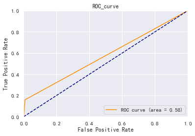
6, Model evaluation
Model evaluation mainly depends on AUC and K-S values
#Model evaluation
from sklearn.metrics import roc_curve, auc
fpr, tpr, threshold = roc_curve(y_test, y_pred)
roc_auc = auc(fpr, tpr)
plt.plot(fpr, tpr, color='darkorange',label='ROC curve (area = %0.2f)' % roc_auc)
plt.plot([0, 1], [0, 1], color='navy',  linestyle='--')
plt.xlim([0.0, 1.0])
plt.ylim([0.0, 1.0])
plt.xlabel('False Positive Rate')
plt.ylabel('True Positive Rate')
plt.title('ROC_curve')
plt.legend(loc="lower right")
plt.show()

roc_auc   #0.5756615527156178
ks
#ks
fig, ax = plt.subplots()
ax.plot(1 - threshold, tpr, label='tpr') # ks curves should be arranged in descending order of prediction probability, so 1-threshold image is required
ax.plot(1 - threshold, fpr, label='fpr')
ax.plot(1 - threshold, tpr-fpr,label='KS')
plt.xlabel('score')
plt.title('KS Curve')
plt.ylim([0.0, 1.0])
plt.figure(figsize=(20,20))
legend = ax.legend(loc='upper left')
plt.show()

max(tpr-fpr)  # 0.1513231054312355
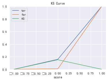
ROC0.58, K-S value is about 0.15, and the modeling effect is general
Why is the score so high, but auc and ks are very low, which is caused by the imbalance of samples
7, Model result transfer score
Assuming that the score is 600 when the good / bad ratio is 20, double the good / bad ratio every 20 points higher
Now let's find the fractional scale corresponding to different woe values of each variable, and we can get:
#Model result transfer score
factor = 20 / np.log(2)
offset = 600 - 20 * np.log(20) / np.log(2)
def get_score(coe,woe,factor):
    scores=[]
    for w in woe:
        score=round(coe*w*factor,0)
        scores.append(score)
    return scores
x1 = get_score(coe[0][0], cut1_woe, factor)
x2 = get_score(coe[0][1], cut2_woe, factor)
x3 = get_score(coe[0][2], cut3_woe, factor)
x4 = get_score(coe[0][3], cut4_woe, factor)
x5 = get_score(coe[0][4], cut5_woe, factor)
x6 = get_score(coe[0][5], cut6_woe, factor)
x7 = get_score(coe[0][6], cut7_woe, factor)
x8 = get_score(coe[0][7], cut8_woe, factor)
x9 = get_score(coe[0][8], cut9_woe, factor)
x10 = get_score(coe[0][9], cut10_woe, factor)
print("Score corresponding to available quota ratio:{}".format(x1))
print("Age corresponding score:{}".format(x2))
print("Overdue 30-59 Score corresponding to the number of Tianbi:{}".format(x3))
print("Score corresponding to debt ratio:{}".format(x4))
print("Score corresponding to monthly income:{}".format(x5))
print("Score corresponding to credit quantity:{}".format(x6))
print("Score corresponding to the number of pen overdue for 90 days:{}".format(x7))
print("Score corresponding to the loan amount of fixed assets:{}".format(x8))
print("Overdue 60-89 Score corresponding to the number of Tianbi:{}".format(x9))
print("Score corresponding to the number of family members:{}".format(x10))
Score corresponding to available quota ratio: [- 22.0, - 21.0, - 5.0, 19.0]
Scores corresponding to age: [7.0, 5.0, 3.0, 2.0, - 0.0, - 5.0, - 11.0, - 14.0]
Scores corresponding to the number of transactions overdue for 30-59 days: [- 7.0, 14.0, 27.0, 37.0, 41.0]
Score corresponding to debt ratio: [- 5.0, - 2.0, 6.0]
Score corresponding to monthly income: [4.0, 1.0, - 2.0, - 4.0]
Score corresponding to credit quantity: [2.0, - 2.0, - 1.0, 0.0]
Scores corresponding to the number of 90 days overdue: [- 6.0, 34.0, 48.0, 56.0, 57.0]
Score corresponding to loan amount of fixed assets: [5.0, - 6.0, - 3.0, 2.0, 16.0]
Scores corresponding to the number of 60-89 days overdue: [- 3.0, 23.0, 35.0, 38.0]
Scores corresponding to the number of family members: [- 1.0, 1.0, 1.0, 2.0, 3.0, 5.0]
It can be seen that the higher the score, the greater the possibility of becoming a bad customer. For example, the older the age, the lower the bad customer rate, the larger the score span of the available quota ratio and the number of overdue transactions, which has a greater impact on the final total score, which confirms the results of the previous exploration and analysis.
8, Calculate total user score
1. Take the boundary division point of automatic box division

cu1=pd.qcut(train_cp["Available limit ratio"],4,labels=False,retbins=True)
bins1=cu1[1]
cu2=pd.qcut(train_cp["Age"],8,labels=False,retbins=True)
bins2=cu2[1]

# bins3=[-1,0,1,3,5,13]
# cut3=pd.cut(train_cp ["30-59 days overdue"], bins3,labels=False)
cu4=pd.qcut(train_cp["Debt ratio"],3,labels=False,retbins=True)
bins4=cu4[1]
cu5=pd.qcut(train_cp["monthly income"],4,labels=False,retbins=True)
bins5=cu5[1]
cu6=pd.qcut(train_cp["Credit quantity"],4,labels=False,retbins=True)
bins6=cu6[1]
2. Sum the scores corresponding to each variable to calculate the total score of each user
#Sum the scores corresponding to each variable to calculate the total score of each user
def compute_score(series,bins,score):
    list = []
    i = 0
    while i < len(series):
        value = series[i]
        j = len(bins) - 2
        m = len(bins) - 2
        while j >= 0:
            if value >= bins[j]:
                j = -1
            else:
                j -= 1
                m -= 1
        list.append(score[m])
        i += 1
    return list
path2=r'F:\\python\\Give-me-some-credit-master\\data\\cs-test.csv'

test1 = pd.read_csv(path2)

test1['x1'] = pd.Series(compute_score(test1['RevolvingUtilizationOfUnsecuredLines'], bins1, x1))
test1['x2'] = pd.Series(compute_score(test1['age'], bins2, x2))
test1['x3'] = pd.Series(compute_score(test1['NumberOfTime30-59DaysPastDueNotWorse'], bins3, x3))
test1['x4'] = pd.Series(compute_score(test1['DebtRatio'], bins4, x4))
test1['x5'] = pd.Series(compute_score(test1['MonthlyIncome'], bins5, x5))
test1['x6'] = pd.Series(compute_score(test1['NumberOfOpenCreditLinesAndLoans'], bins6, x6))
test1['x7'] = pd.Series(compute_score(test1['NumberOfTimes90DaysLate'], bins7, x7))
test1['x8'] = pd.Series(compute_score(test1['NumberRealEstateLoansOrLines'], bins8, x8))
test1['x9'] = pd.Series(compute_score(test1['NumberOfTime60-89DaysPastDueNotWorse'], bins9, x9))
test1['x10'] = pd.Series(compute_score(test1['NumberOfDependents'], bins10, x10))
test1['Score'] = test1['x1']+test1['x2']+test1['x3']+test1['x4']+test1['x5']+test1['x6']+test1['x7']+test1['x8']+test1['x9']+test1['x10']+600
test1.to_csv(r'F:\\python\\Give-me-some-credit-master\\data\\ScoreData.csv', index=False)
Article reprint: https://www.cnblogs.com/daliner/p/10268350.html
All codes:

# -*- coding: utf-8 -*-
"""
Created on Tue Aug 11 14:09:20 2020

@author: Admin
"""

#Import module
import pandas as pd
import numpy as np
from scipy import stats
import seaborn as sns
import matplotlib.pyplot as plt
%matplotlib inline
plt.rc("font",family="SimHei",size="12")  #Solve the problem that Chinese cannot be displayed

#Import data
train=pd.read_csv('F:\\python\\Give-me-some-credit-master\\data\\cs-training.csv')

#Simple view data
train.info()

#Data viewing of the first three rows and the last three rows
b=train.head(3).append(train.tail(3))

#shape
train.shape  #(150000, 11)

#Convert English fields to Chinese field names for easy understanding
states={'Unnamed: 0':'id',
        'SeriousDlqin2yrs':'Good and bad customers',
        'RevolvingUtilizationOfUnsecuredLines':'Available limit ratio',
        'age':'Age',
        'NumberOfTime30-59DaysPastDueNotWorse':'Overdue 30-59 Tianbi number',
        'DebtRatio':'Debt ratio',
        'MonthlyIncome':'monthly income',
        'NumberOfOpenCreditLinesAndLoans':'Credit quantity',
        'NumberOfTimes90DaysLate':'Number of transactions overdue for 90 days',
        'NumberRealEstateLoansOrLines':'Fixed asset loans',
        'NumberOfTime60-89DaysPastDueNotWorse':'Overdue 60-89 Tianbi number',
        'NumberOfDependents':'Number of family members'}
train.rename(columns=states,inplace=True)

#catalog index
train=train.set_index('id',drop=True)

#descriptive statistics
train.describe()

#Check the missing condition of each column
train.isnull().sum()
#Check the missing proportion
train.isnull().sum()/len(train)
#Missing value visualization
missing=train.isnull().sum()
missing[missing>0].sort_values().plot.bar()  #Take out and sort those greater than 0

#Keep original data
train_cp=train.copy()

#Monthly income uses the average to fill in the missing value
train_cp.fillna({'monthly income':train_cp['monthly income'].mean()},inplace=True)
train_cp.isnull().sum()

#Lines with missing number of family members are removed
train_cp=train_cp.dropna()
train_cp.shape   #(146076, 11)

#View outliers
#Draw box diagram
for col in train_cp.columns:
    plt.boxplot(train_cp[col])
    plt.title(col)
    plt.show()

#Outlier handling
train_cp=train_cp[train_cp['Available limit ratio']<1]
train_cp=train_cp[train_cp['Age']>0]
train_cp=train_cp[train_cp['Overdue 30-59 Tianbi number']<80]
train_cp=train_cp[train_cp['Overdue 60-89 Tianbi number']<80]
train_cp=train_cp[train_cp['Number of transactions overdue for 90 days']<80]
train_cp=train_cp[train_cp['Fixed asset loans']<50]
train_cp=train_cp[train_cp['Debt ratio']<5000]
train_cp.shape  #(141180, 11)

#Univariate analysis
#Good and bad users
train_cp.info()
train_cp['Good and bad customers'].value_counts()
train_cp['Good and bad customers'].value_counts()/len(train_cp)
train_cp['Good and bad customers'].value_counts().plot.bar()

#Available limit ratio and debt ratio
train_cp['Available limit ratio'].plot.hist()
train_cp['Debt ratio'].plot.hist()
#The data with a debt ratio greater than 1 has too much impact
a=train_cp['Debt ratio']
a[a<=1].plot.hist()

#30-59 days overdue, 90 days overdue, 60-89 days overdue
for i,col in enumerate(['Overdue 30-59 Tianbi number','Number of transactions overdue for 90 days','Overdue 60-89 Tianbi number']):
    plt.subplot(1,3,i+1)
    train_cp[col].value_counts().plot.bar()
    plt.title(col)


train_cp['Overdue 30-59 Tianbi number'].value_counts().plot.bar()
train_cp['Number of transactions overdue for 90 days'].value_counts().plot.bar()
train_cp['Overdue 60-89 Tianbi number'].value_counts().plot.bar()


#Age
train_cp['Age'].plot.hist()

#monthly income
train_cp['monthly income'].plot.hist()
sns.distplot(train_cp['monthly income'])
#The influence of super outliers is too great. We take the data less than 5w to draw the graph
a=train_cp['monthly income']
a[a<=50000].plot.hist()

#If it is found that there are not many less than 50000, take 2w
a=train_cp['monthly income']
a[a<=20000].plot.hist()

#Credit quantity
train_cp['Credit quantity'].value_counts().plot.bar()
sns.distplot(train_cp['Credit quantity'])

#Fixed asset loans
train_cp['Fixed asset loans'].value_counts().plot.bar()
sns.distplot(train_cp['Fixed asset loans'])

#Number of family members
train_cp['Number of family members'].value_counts().plot.bar()
sns.distplot(train_cp['Number of family members'])

#Univariate and y-value visualization
#Available quota ratio, debt ratio, age and monthly income need to be separated
#Available limit ratio
train_cp['Available limit ratio_cut']=pd.cut(train_cp['Available limit ratio'],5)
pd.crosstab(train_cp['Available limit ratio_cut'],train_cp['Good and bad customers']).plot(kind="bar")
a=pd.crosstab(train_cp['Available limit ratio_cut'],train_cp['Good and bad customers'])
a['Proportion of bad users']=a[1]/(a[0]+a[1])
a['Proportion of bad users'].plot()

#Debt ratio
cut=[-1,0.2,0.4,0.6,0.8,1,1.5,2,5,10,5000]
train_cp['Debt ratio_cut']=pd.cut(train_cp['Debt ratio'],bins=cut)
pd.crosstab(train_cp['Debt ratio_cut'],train_cp['Good and bad customers']).plot(kind="bar")
a=pd.crosstab(train_cp['Debt ratio_cut'],train_cp['Good and bad customers'])
a['Proportion of bad users']=a[1]/(a[0]+a[1])
a['Proportion of bad users'].plot()

#Age
cut=[0,30,40,50,60,100]
train_cp['Age_cut']=pd.cut(train_cp['Age'],bins=cut)
pd.crosstab(train_cp['Age_cut'],train_cp['Good and bad customers']).plot(kind="bar")
a=pd.crosstab(train_cp['Age_cut'],train_cp['Good and bad customers'])
a['Proportion of bad users']=a[1]/(a[0]+a[1])
a['Proportion of bad users'].plot()

#monthly income
cut=[0,3000,5000,7000,10000,15000,30000,1000000]
train_cp['monthly income_cut']=pd.cut(train_cp['monthly income'],bins=cut)
pd.crosstab(train_cp['monthly income_cut'],train_cp['Good and bad customers']).plot(kind="bar")
a=pd.crosstab(train_cp['monthly income_cut'],train_cp['Good and bad customers'])
a['Proportion of bad users']=a[1]/(a[0]+a[1])
a['Proportion of bad users'].plot()

#30-59 days overdue, 90 days overdue, 60-89 days overdue \ amount of credit \ amount of fixed asset loans \ number of family members
#30-59 days overdue
pd.crosstab(train_cp['Overdue 30-59 Tianbi number'],train_cp['Good and bad customers']).plot(kind="bar")
a=pd.crosstab(train_cp['Overdue 30-59 Tianbi number'],train_cp['Good and bad customers'])
a['Proportion of bad users']=a[1]/(a[0]+a[1])
a['Proportion of bad users'].plot()

#Number of transactions overdue for 90 days
pd.crosstab(train_cp['Number of transactions overdue for 90 days'],train_cp['Good and bad customers']).plot(kind="bar")
a=pd.crosstab(train_cp['Number of transactions overdue for 90 days'],train_cp['Good and bad customers'])
a['Proportion of bad users']=a[1]/(a[0]+a[1])
a['Proportion of bad users'].plot()

#60-89 days overdue
pd.crosstab(train_cp['Overdue 60-89 Tianbi number'],train_cp['Good and bad customers']).plot(kind="bar")
a=pd.crosstab(train_cp['Overdue 60-89 Tianbi number'],train_cp['Good and bad customers'])
a['Proportion of bad users']=a[1]/(a[0]+a[1])
a['Proportion of bad users'].plot()

#Credit quantity
cut=[-1,0,1,2,3,4,5,10,15,100]
train_cp['Credit quantity_cut']=pd.cut(train_cp['monthly income'],bins=cut)
pd.crosstab(train_cp['Credit quantity_cut'],train_cp['Good and bad customers']).plot(kind="bar")
a=pd.crosstab(train_cp['Credit quantity_cut'],train_cp['Good and bad customers'])
a['Proportion of bad users']=a[1]/(a[0]+a[1])
a['Proportion of bad users'].plot()

#Fixed asset loans
pd.crosstab(train_cp['Fixed asset loans'],train_cp['Good and bad customers']).plot(kind="bar")
a=pd.crosstab(train_cp['Fixed asset loans'],train_cp['Good and bad customers'])
a['Proportion of bad users']=a[1]/(a[0]+a[1])
a['Proportion of bad users'].plot()


#Number of family members
pd.crosstab(train_cp['Number of family members'],train_cp['Good and bad customers']).plot(kind="bar")
a=pd.crosstab(train_cp['Number of family members'],train_cp['Good and bad customers'])
a['Proportion of bad users']=a[1]/(a[0]+a[1])
a['Proportion of bad users'].plot()


#Correlation between variables
train_cp.corr()['Good and bad customers'].sort_values(ascending = False).plot(kind='bar')
plt.figure(figsize=(20,16))
corr=train_cp.corr()
sns.heatmap(corr, xticklabels=corr.columns, yticklabels=corr.columns,
                 linewidths=0.2, cmap="YlGnBu",annot=True)

#woe sub box
cut1=pd.qcut(train_cp["Available limit ratio"],4,labels=False)
cut2=pd.qcut(train_cp["Age"],8,labels=False)
bins3=[-1,0,1,3,5,13]
cut3=pd.cut(train_cp["Overdue 30-59 Tianbi number"],bins3,labels=False)
cut4=pd.qcut(train_cp["Debt ratio"],3,labels=False)
cut5=pd.qcut(train_cp["monthly income"],4,labels=False)
cut6=pd.qcut(train_cp["Credit quantity"],4,labels=False)
bins7=[-1, 0, 1, 3,5, 20]
cut7=pd.cut(train_cp["Number of transactions overdue for 90 days"],bins7,labels=False)
bins8=[-1, 0,1,2, 3, 33]
cut8=pd.cut(train_cp["Fixed asset loans"],bins8,labels=False)
bins9=[-1, 0, 1, 3, 12]
cut9=pd.cut(train_cp["Overdue 60-89 Tianbi number"],bins9,labels=False)
bins10=[-1, 0, 1, 2, 3, 5, 21]
cut10=pd.cut(train_cp["Number of family members"],bins10,labels=False)

#woe calculation
rate=train_cp["Good and bad customers"].sum()/(train_cp["Good and bad customers"].count()-train_cp["Good and bad customers"].sum())  #rate = bad / (total bad)
def get_woe_data(cut):
    grouped=train_cp["Good and bad customers"].groupby(cut,as_index = True).value_counts()
    woe=np.log(grouped.unstack().iloc[:,1]/grouped.unstack().iloc[:,0]/rate)
    return woe
cut1_woe=get_woe_data(cut1)
cut2_woe=get_woe_data(cut2)
cut3_woe=get_woe_data(cut3)
cut4_woe=get_woe_data(cut4)
cut5_woe=get_woe_data(cut5)
cut6_woe=get_woe_data(cut6)
cut7_woe=get_woe_data(cut7)
cut8_woe=get_woe_data(cut8)
cut9_woe=get_woe_data(cut9)
cut10_woe=get_woe_data(cut10)

l=[cut1_woe,cut2_woe,cut3_woe,cut4_woe,cut5_woe,cut6_woe,cut7_woe,cut8_woe,cut9_woe,cut10_woe]
for i,col in enumerate(l):
    col.plot()


#iv value calculation
def get_IV_data(cut,cut_woe):
    grouped=train_cp["Good and bad customers"].groupby(cut,as_index = True).value_counts()
    cut_IV=((grouped.unstack().iloc[:,1]/train_cp["Good and bad customers"].sum()-grouped.unstack().iloc[:,0]/(train_cp["Good and bad customers"].count()-train_cp["Good and bad customers"].sum()))*cut_woe).sum()
    return cut_IV
#Calculate the IV value of each group
cut1_IV=get_IV_data(cut1,cut1_woe)
cut2_IV=get_IV_data(cut2,cut2_woe)
cut3_IV=get_IV_data(cut3,cut3_woe)
cut4_IV=get_IV_data(cut4,cut4_woe)
cut5_IV=get_IV_data(cut5,cut5_woe)
cut6_IV=get_IV_data(cut6,cut6_woe)
cut7_IV=get_IV_data(cut7,cut7_woe)
cut8_IV=get_IV_data(cut8,cut8_woe)
cut9_IV=get_IV_data(cut9,cut9_woe)
cut10_IV=get_IV_data(cut10,cut10_woe)
IV=pd.DataFrame([cut1_IV,cut2_IV,cut3_IV,cut4_IV,cut5_IV,cut6_IV,cut7_IV,cut8_IV,cut9_IV,cut10_IV],index=['Available limit ratio','Age','Overdue 30-59 Tianbi number','Debt ratio','monthly income','Credit quantity','Number of transactions overdue for 90 days','Fixed asset loans','Overdue 60-89 Tianbi number','Number of family members'],columns=['IV'])
iv=IV.plot.bar(color='b',alpha=0.3,rot=30,figsize=(10,5),fontsize=(10))
iv.set_title('Characteristic variables and IV Value distribution diagram',fontsize=(15))
iv.set_xlabel('Characteristic variable',fontsize=(15))
iv.set_ylabel('IV',fontsize=(15))

#woe conversion
df_new=pd.DataFrame()   #New df_new stores the data converted by woe
def replace_data(cut,cut_woe):
    a=[]
    for i in cut.unique():
        a.append(i)
        a.sort()
    for m in range(len(a)):
        cut.replace(a[m],cut_woe.values[m],inplace=True)
    return cut
df_new["Good and bad customers"]=train_cp["Good and bad customers"]
df_new["Available limit ratio"]=replace_data(cut1,cut1_woe)
df_new["Age"]=replace_data(cut2,cut2_woe)
df_new["Overdue 30-59 Tianbi number"]=replace_data(cut3,cut3_woe)
df_new["Debt ratio"]=replace_data(cut4,cut4_woe)
df_new["monthly income"]=replace_data(cut5,cut5_woe)
df_new["Credit quantity"]=replace_data(cut6,cut6_woe)
df_new["Number of transactions overdue for 90 days"]=replace_data(cut7,cut7_woe)
df_new["Fixed asset loans"]=replace_data(cut8,cut8_woe)
df_new["Overdue 60-89 Tianbi number"]=replace_data(cut9,cut9_woe)
df_new["Number of family members"]=replace_data(cut10,cut10_woe)
df_new.head()

#model training
from sklearn.linear_model import LogisticRegression
from sklearn.model_selection import train_test_split
x=df_new.iloc[:,1:]
y=df_new.iloc[:,:1]
x_train,x_test,y_train,y_test=train_test_split(x,y,test_size=0.6,random_state=0)
model=LogisticRegression()
clf=model.fit(x_train,y_train)
print('Test results:{}'.format(clf.score(x_test,y_test)))

#coefficient
coe=clf.coef_        #Feature weight coefficient, which will be used later when converted to scoring rules
coe

#Score of test set
y_pred=clf.predict(x_test)

#Model evaluation
from sklearn.metrics import roc_curve, auc
fpr, tpr, threshold = roc_curve(y_test, y_pred)
roc_auc = auc(fpr, tpr)
plt.plot(fpr, tpr, color='darkorange',label='ROC curve (area = %0.2f)' % roc_auc)
plt.plot([0, 1], [0, 1], color='navy',  linestyle='--')
plt.xlim([0.0, 1.0])
plt.ylim([0.0, 1.0])
plt.xlabel('False Positive Rate')
plt.ylabel('True Positive Rate')
plt.title('ROC_curve')
plt.legend(loc="lower right")
plt.show()

roc_auc   #0.5756615527156178

#ks
fig, ax = plt.subplots()
ax.plot(1 - threshold, tpr, label='tpr') # ks curves should be arranged in descending order of prediction probability, so 1-threshold image is required
ax.plot(1 - threshold, fpr, label='fpr')
ax.plot(1 - threshold, tpr-fpr,label='KS')
plt.xlabel('score')
plt.title('KS Curve')
plt.ylim([0.0, 1.0])
plt.figure(figsize=(20,20))
legend = ax.legend(loc='upper left')
plt.show()

max(tpr-fpr)  # 0.1513231054312355


#Model result transfer score
factor = 20 / np.log(2)
offset = 600 - 20 * np.log(20) / np.log(2)
def get_score(coe,woe,factor):
    scores=[]
    for w in woe:
        score=round(coe*w*factor,0)
        scores.append(score)
    return scores
x1 = get_score(coe[0][0], cut1_woe, factor)
x2 = get_score(coe[0][1], cut2_woe, factor)
x3 = get_score(coe[0][2], cut3_woe, factor)
x4 = get_score(coe[0][3], cut4_woe, factor)
x5 = get_score(coe[0][4], cut5_woe, factor)
x6 = get_score(coe[0][5], cut6_woe, factor)
x7 = get_score(coe[0][6], cut7_woe, factor)
x8 = get_score(coe[0][7], cut8_woe, factor)
x9 = get_score(coe[0][8], cut9_woe, factor)
x10 = get_score(coe[0][9], cut10_woe, factor)
print("Score corresponding to available quota ratio:{}".format(x1))
print("Age corresponding score:{}".format(x2))
print("Overdue 30-59 Score corresponding to the number of Tianbi:{}".format(x3))
print("Score corresponding to debt ratio:{}".format(x4))
print("Score corresponding to monthly income:{}".format(x5))
print("Score corresponding to credit quantity:{}".format(x6))
print("Score corresponding to the number of pen overdue for 90 days:{}".format(x7))
print("Score corresponding to the loan amount of fixed assets:{}".format(x8))
print("Overdue 60-89 Score corresponding to the number of Tianbi:{}".format(x9))
print("Score corresponding to the number of family members:{}".format(x10))

#1. Take the boundary division point of automatic box division
cu1=pd.qcut(train_cp["Available limit ratio"],4,labels=False,retbins=True)
bins1=cu1[1]
cu2=pd.qcut(train_cp["Age"],8,labels=False,retbins=True)
bins2=cu2[1]

# bins3=[-1,0,1,3,5,13]
# cut3=pd.cut(train_cp ["30-59 days overdue"], bins3,labels=False)
cu4=pd.qcut(train_cp["Debt ratio"],3,labels=False,retbins=True)
bins4=cu4[1]
cu5=pd.qcut(train_cp["monthly income"],4,labels=False,retbins=True)
bins5=cu5[1]
cu6=pd.qcut(train_cp["Credit quantity"],4,labels=False,retbins=True)
bins6=cu6[1]


#Sum the scores corresponding to each variable to calculate the total score of each user
def compute_score(series,bins,score):
    list = []
    i = 0
    while i < len(series):
        value = series[i]
        j = len(bins) - 2
        m = len(bins) - 2
        while j >= 0:
            if value >= bins[j]:
                j = -1
            else:
                j -= 1
                m -= 1
        list.append(score[m])
        i += 1
    return list
path2=r'F:\\python\\Give-me-some-credit-master\\data\\cs-test.csv'

test1 = pd.read_csv(path2)

test1['x1'] = pd.Series(compute_score(test1['RevolvingUtilizationOfUnsecuredLines'], bins1, x1))
test1['x2'] = pd.Series(compute_score(test1['age'], bins2, x2))
test1['x3'] = pd.Series(compute_score(test1['NumberOfTime30-59DaysPastDueNotWorse'], bins3, x3))
test1['x4'] = pd.Series(compute_score(test1['DebtRatio'], bins4, x4))
test1['x5'] = pd.Series(compute_score(test1['MonthlyIncome'], bins5, x5))
test1['x6'] = pd.Series(compute_score(test1['NumberOfOpenCreditLinesAndLoans'], bins6, x6))
test1['x7'] = pd.Series(compute_score(test1['NumberOfTimes90DaysLate'], bins7, x7))
test1['x8'] = pd.Series(compute_score(test1['NumberRealEstateLoansOrLines'], bins8, x8))
test1['x9'] = pd.Series(compute_score(test1['NumberOfTime60-89DaysPastDueNotWorse'], bins9, x9))
test1['x10'] = pd.Series(compute_score(test1['NumberOfDependents'], bins10, x10))
test1['Score'] = test1['x1']+test1['x2']+test1['x3']+test1['x4']+test1['x5']+test1['x6']+test1['x7']+test1['x8']+test1['x9']+test1['x10']+600
test1.to_csv(r'F:\\python\\Give-me-some-credit-master\\data\\ScoreData.csv', index=False)
Reprint https://www.cnblogs.com/cgmcoding/p/13491940.html
That's all for python,
Welcome to register< python financial risk control scorecard model and data analysis micro professional course >, learn more about it.