1 Introduction to Wavelet Analysis

Compared with the Fourier transform ratio, both the wavelet transform and the short-time Fourier transform have the same advantages, that is, the signal can be observed in both time and frequency domains.Therefore, the analysis of unsteady signals based on wavelet transform is very useful.

For articles on short-time Fourier transforms, see the following:
Short-time Fourier transform spectrogram for matlab time-frequency analysis
https://blog.csdn.net/weixin_42943114/article/details/88735799

Compared with short-time Fourier transform, wavelet transform has the characteristics of window adaptive, that is, high resolution (but poor frequency resolution) of high frequency signal and high resolution (but poor time resolution) of low frequency signal. In engineering, it is often concerned about low frequency and high frequency occurrence time, so it has been widely used in recent years.

Mathematically, wavelet has the advantage of orthogonalization and is widely used.
However, this article only discusses how to use matlab to implement time-frequency analysis of cwt

2 Basic Principles of Wavelet Analysis

The meaning of wavelet is that it decays fast in time and is shorter than Fourier's sinusoidal wave.
A typical morlet wavelet is shown below: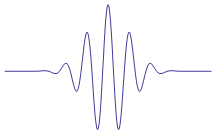

matlab has many own wavelet functions, which can be viewed by wavemngr('read', 1) and related information by waveinfo.

In time domain, the wavelet coefficients can be obtained by comparing the window signals at different locations one by one through the movement of the wavelet in time. The larger the wavelet coefficients, the better the fit between the wavelet and the signal at that segment.The convolution of the wavelet function with the window signal is used in the calculation as the wavelet coefficients under the window.The length of the window is the same as that of the wavelet.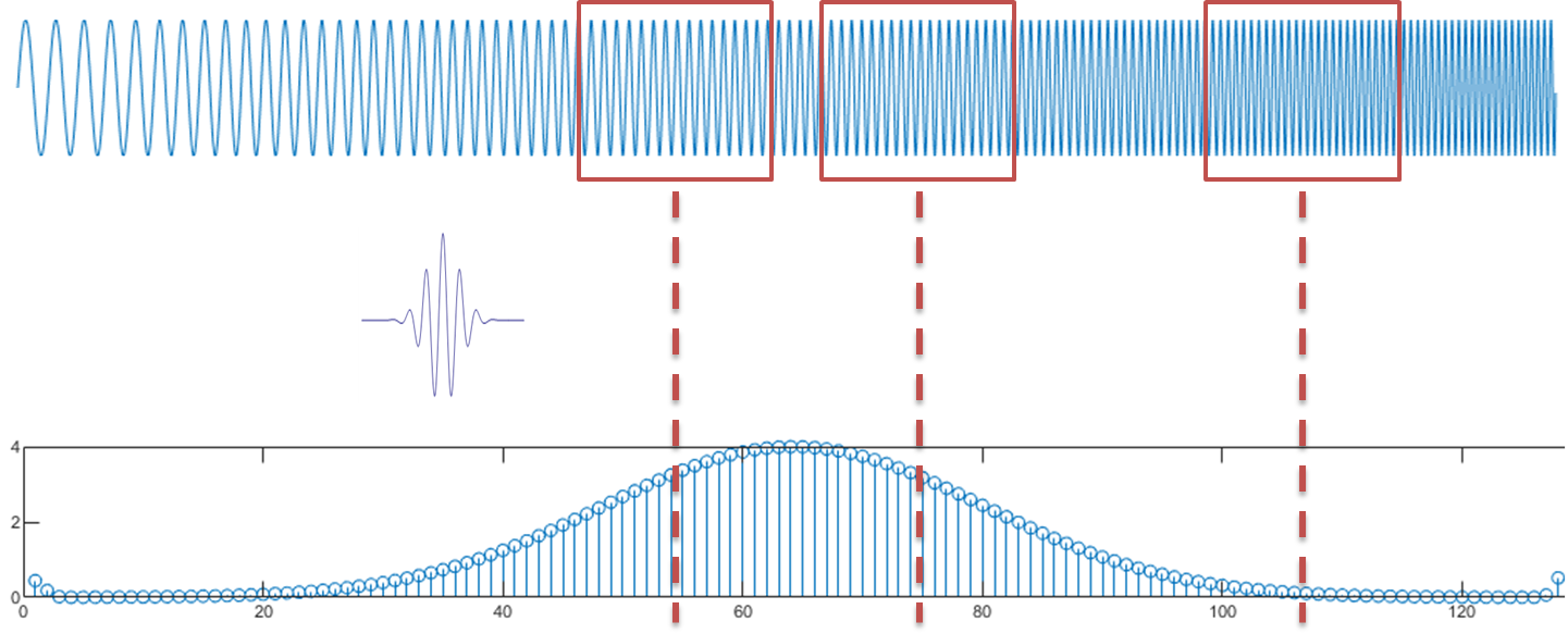

In the frequency domain, the wavelet coefficients at different frequencies are achieved by stretching or compressing the length of the wavelet to change the length and frequency of the wavelet.Correspondingly, the window length will also change with the length of the wavelet.Because the wavelet is compressed at high frequencies, the time window becomes narrower and the time resolution is higher.

By combining the wavelet coefficients at different frequencies, the time-frequency transformation wavelet coefficients map is obtained.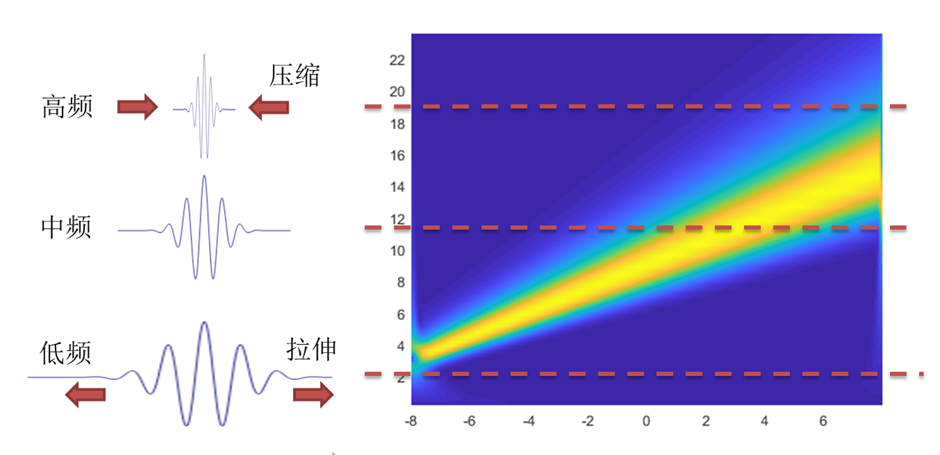

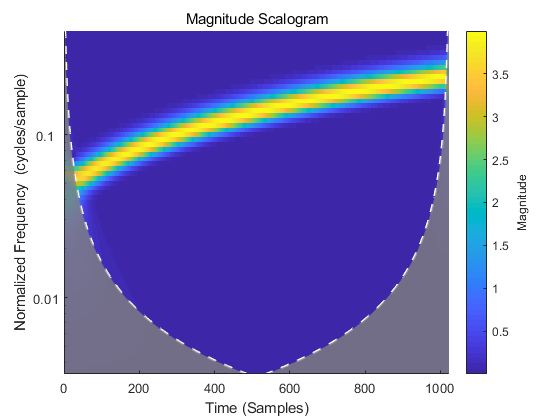
As you can see from the graph, the frequency resolution at low frequencies is better than at high frequencies.Wavelet time-frequency maps are characterized by overall high and thin at high frequencies and short and wide at low frequencies.

In wavelet, the frequency f of a wavelet is generally measured by a scale scale, and the conversion relationship between the two is:
scale∗f=Fs∗wcf scale * f=Fs * wcf scale∗f=Fs∗wcf
In the formula, Fs represents the sampling frequency of the signal, wcf is the center frequency of the wavelet transform (wave central freq), which can be queried by centfrq(wavename) in matlab.

matlab implementation of 3 cwt

matlab comes with two implementations, one is the function cwt launched in the 2006 version and the other is the function cwt launched in the 2016 version.The two functions have the same name and different usage.
(I don't know why this is the case either.)--|)

Since the names are the same, in use, you can only distinguish between input and output formats if you want to call different versions.

The old version of cwt was used as:

coefs = cwt(x,scales,'wname')

The new version of cwt uses:

[wt,f] = cwt(x,wname,fs)

The most obvious difference is that the new version removes the ability to customize scale functions.The new version also updates and replaces some of the wavelet functions.The old version supports wavelets like'haar','db','sym','cmor','mexh','gaus','bior', and the new version supports'morse','amor'and'bump' wavelets.

The new version of the wavelet function uses the following:

% Define signal information
fs=2^6;    %sampling frequency
dt=1/fs;    %Time accuracy
timestart=-8;
timeend=8;
t=(0:(timeend-timestart)/dt-1)*dt+timestart;
L=length(t);

z=4*sin(2*pi*linspace(6,12,L).*t);

%matlab In-band Wavelet Transform
%new version
figure(1)
[wt,f,coi] = cwt(z,'amor',fs);
pcolor(t,f,abs(wt));shading interp

The old version of the wavelet function uses the following:
cmor wavelet and frequency scaling are used here.

% Define signal information
fs=2^6;    %sampling frequency
dt=1/fs;    %Time accuracy
timestart=-8;
timeend=8;
t=(0:(timeend-timestart)/dt-1)*dt+timestart;
L=length(t);

z=4*sin(2*pi*linspace(6,12,L).*t);
%Old Version
wavename='cmor1-3'; %Variable parameters, respectively cmor Of
%An example of frequency scaling
fmin=2;
fmax=20;
df=0.1;

f=fmin:df:fmax-df;%Expected frequency
wcf=centfrq(wavename); %Center Frequency of Wavelet
scal=fs*wcf./f;%Using frequency conversion scales
coefs = cwt(z,scal,wavename);
figure(2)
pcolor(t,f,abs(coefs));shading interp

For the selection of cmor wavelet Fc and Fb, it can be assumed that the final result only depends on the product size of Fc*Fb.In practical application, the specific value needs to be selected according to the final effect.

The coefs wavelet coefficients obtained by cmor wavelet transform are a complex matrix, the absolute value abs() represents the amplitude of the signal, and the angle() represents the phase of the signal.Generally, the real part of the wavelet coefficients, real(), is used to represent both positive and negative changes in the signal.

In fact, the principle of cwt is very simple, that is, to deconvolute each window with different scales of wavelets and get the matrix of wavelet coefficients.So according to the principle, the wavelet transform can be programmed by itself.

The cwt functions you have programmed are as follows, where the main algorithms are referenced in the official matlab documentation.Here I still use the cmor wavelet as an example. The morlet function formula can be queried or called with the cmorwavf() function:

fs=2^6;    %sampling frequency
dt=1/fs;    %Time accuracy
timestart=-8;
timeend=8;
t=(0:(timeend-timestart)/dt-1)*dt+timestart;
L=length(t);
z=4*sin(2*pi*linspace(6,12,L).*t);

%Define calculation range and precision
fmin=2;
fmax=20;
df=0.1;
totalscal=(fmax-fmin)/df;
f=fmin:df:fmax-df;%Expected frequency
wcf=centfrq(wavename); %Center Frequency of Wavelet
scal=fs*wcf./f;

%Self-implemented Wavelet Functions
coefs2=cwt_cmor(z,1,3,f,fs);
figure(3)
pcolor(t,f,abs(coefs2));shading interp


%Following is the function
function coefs=cwt_cmor(z,Fb,Fc,f,fs)
%1 Preparation of Normalized Signal for Wavelet
z=z(:)';%Force to become y Vector, avoid previous errors
L=length(z);
%2 Calculating scale
scal=fs*Fc./f;

%3 Computational Wavelet
shuaijian=0.001;%Take Wavelet Decay Length of 1%
tlow2low=sqrt(Fb*log(1/shuaijian));%unilateral cmor Decay to 1%Time duration, scream cmor Expression

%3 Integral function of wavelet
iter=10;%Interval Partition Precision of Wavelet Functions
xWAV=linspace(-tlow2low,tlow2low,2^iter);
stepWAV = xWAV(2)-xWAV(1);
val_WAV=cumsum(cmorwavf(-tlow2low,tlow2low,2^iter,Fb,Fc))*stepWAV;
%Pre-convolution preparation
xWAV = xWAV-xWAV(1);
xMaxWAV = xWAV(end);
coefs     = zeros(length(scal),L);%Preset coefs

%4 Convolution of Wavelet and Signal
for k = 1:length(scal)    %One scal A line
    a_SIG = scal(k); %a Is the scale function of this line

    j = 1+floor((0:a_SIG*xMaxWAV)/(a_SIG*stepWAV));
        %j The maximum value is determined, and the larger the scale, the closer the division.Equivalent to stretching a small wave longer.
    if length(j)==1 , j = [1 1]; end
    
    waveinscal = fliplr(val_WAV(j));%Extend the integral value to j Interval, then invert left and right. f Integral Wavelet Function for Current Scale
    
    %5 The most important step wkeep1 take diff(wconv1(ySIG,f))The mile length is lenSIG Middle Section
    %conv(ySIG,f)Convolution.
    coefs(k,:) = -sqrt(a_SIG)*wkeep1(diff(conv2(z,waveinscal, 'full')),L);
    %
end
end

The output is as follows, and you can see that the result is basically the same as that obtained by the function that comes with matlab.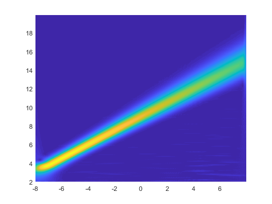

Edge Effect and Impact Cone of 4 cwt

With its own cwt function, the influence cone can be easily drawn.

cwt(z)

Because the wavelet coefficients are convoluted by window functions and wavelets in the wavelet computation, when the window is on the edge of the signal, there will be some no signal in the window.At this point, matlab zeroes this incomplete part of the window, making it long enough.

At this time, because the signal is compelled to zero at the edge, the signal will be distorted, which is represented in the time-frequency diagram as a wider frequency and lower signal strength.When severe, even the whole low frequency part will be distorted.This is the edge effect of cwt.

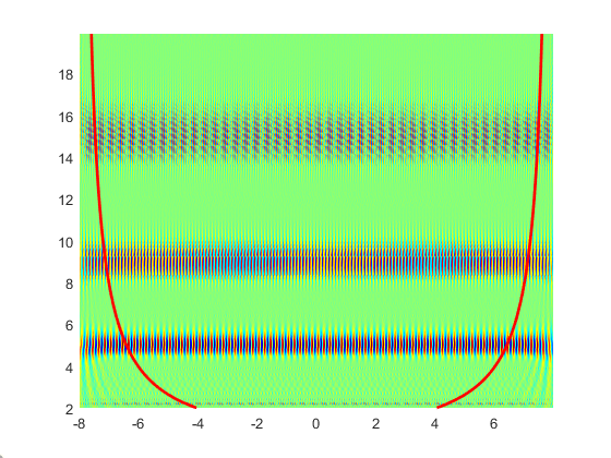
In order to determine the influence of edge effect, an influence curve is drawn. The signal inside the curve has little or no influence, while the signal outside the curve has greater influence.The curve is like a cone, with the high frequencies near the sides and the low frequencies near the middle, so it is also called the influence cone.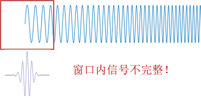

So according to the principle of edge effect, it is known that the small influence range at high frequencies is because the wavelet is compressed at high frequencies, so the window is narrower.Wavelets are stretched at low frequencies, so they correspond to wider windows.The length of the window is the same as that of the wavelet.

There are many ways to evaluate the impact range. For convenience, I draw the impact cone directly using the half-length of the wavelet as the impact range.Specific ideas are as follows, I think that more than half the length of the wavelet is distorted, and then calculate the wavelet length of each point by frequency, and then draw the lines on the graph.

The code is as follows, still taking the cmor wavelet as an example, in order to reflect the phase effect, real() is used here:

%Wavelet Transform Display
clear
fs=2^6;    %sampling frequency
dt=1/fs;    %Time accuracy
timestart=-8;
timeend=8;
t=(0:(timeend-timestart)/dt-1)*dt+timestart;
L=length(t);

z=sin(2*pi*5.*t)+sin(2*pi*9.*t)+sin(2*pi*15.*t);

%Define Scope
wavename='cmor1-3'; %Variable parameters
fmin=2;
fmax=20;
df=0.1;
totalscal=(fmax-fmin)/df;
f=fmin:df:fmax-df;%Expected frequency
wcf=centfrq(wavename); %Center Frequency of Wavelet
scal=fs*wcf./f;

%Old Version
coefs = cwt(z,scal,wavename);
figure(2)
pcolor(t,f,real(coefs));shading interp

tlow2low=sqrt(1*log(1/0.001));%unilateral cmor Decay to 1%Time length of hour
tcoi41=tlow2low*scal;%Wavelet Half Length
bur=(tcoi41<L/2);
fcoi4=f(bur);
tcoi41=tcoi41(bur);
tcoi42=-tcoi41+L;
hold on
plot(tcoi41/fs+timestart,fcoi4,'r','LineWidth',2)
plot(tcoi42/fs+timestart,fcoi4,'r','LineWidth',2)
hold off

Reconfiguration of 5 cwt-icwt

If the default wavelet of the new version of matlab is used, the icwt of the wavelet coefficients after cwt can be used directly.

load mtlb;
wt = cwt(mtlb);
xrec = icwt(wt);

For morlet wavelets, the reconstruction can be achieved by direct sum(real(coefs),1).However, it is best to use the default scale here, otherwise duplicate overlays will cause problems with the amplitude.

See the help documentation for specific usage.

6 wsst to increase cwt resolution

wsst can significantly improve the frequency resolution of cwt.The specific usage is as follows:

clear
fs=2^6;    %sampling frequency
dt=1/fs;    %Time accuracy
timestart=-8;
timeend=8;
t=(0:(timeend-timestart)/dt-1)*dt+timestart;
L=length(t);
z=4*sin(2*pi*linspace(6,12,L).*t);

[sst,f] = wsst(z,fs);
figure(4)
pcolor(t,f,abs(sst));shading interp

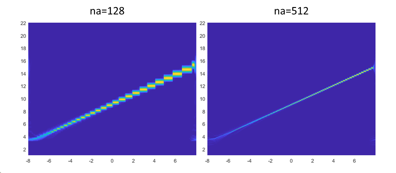
The comparison with normal cwt is as follows: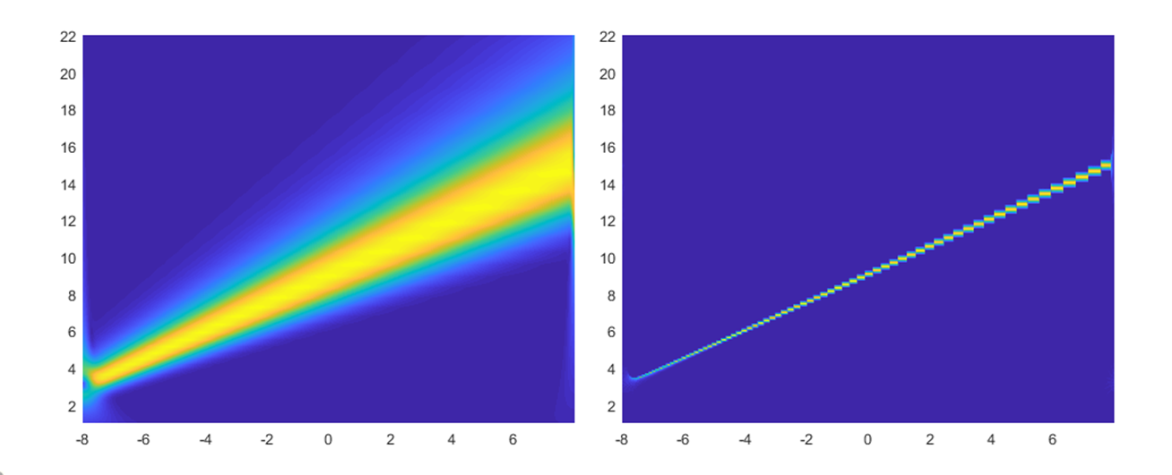

The left is the time-frequency diagram of cwt, and the right is the time-frequency diagram of wsst.
wsst can also be refactored using iwsst, which can be found in iwsst's help documentation.

If you want to improve the accuracy of wsst, you can select wsst in matlab, then Ctrl+D enters the code interface of wsst, and force the na parameter inside to be larger.

This is done by adding a na=512 after the code below (not necessarily 512 here, but by zooming in appropriately based on the actual value of na, in my example here, na=288).Backup is recommended if you are afraid of errors.

na = noct*params.nv;
na=512

The advantage of this is that the decomposition accuracy is significantly improved without affecting the results of iwsst.