Cyclic Neural Network Learning

Circular Neural Network RNN

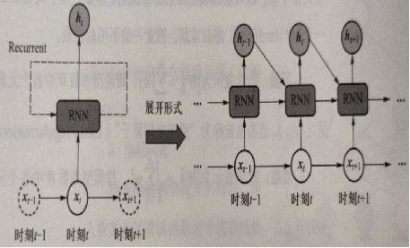
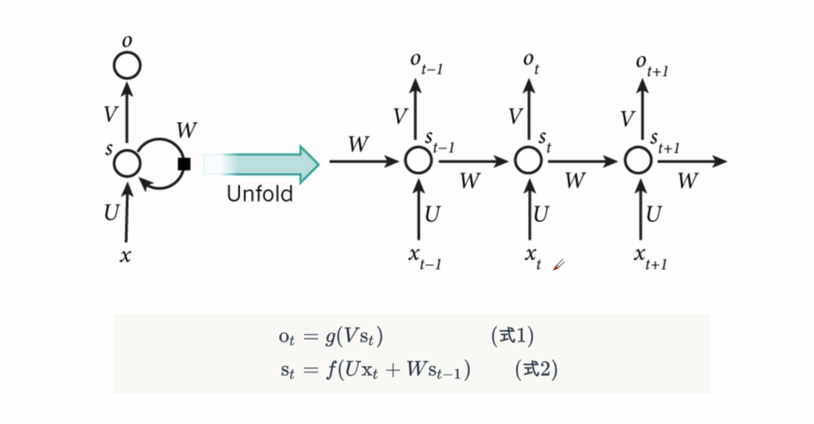
At time t, once the current input data x_is obtained T, the recurrent neural network combines the implicit coding _obtained from the previous moment t_1 T_1, produces the implicit encoding of the current moment as follows__ T:
ℎ_t=Φ(U×x_t+W×ℎ_t−1)

Here Φ () is an activation function, which can be either a Sigmoid or a Tanh activation function, enabling the model to forget extraneous information and update memory content at the same time. U and W are model parameters. As you can see here, the implicitly coded output of the current moment_ t is not only related to the current input data x_t-related, with existing "memory" of the network__ t_1 also has an inseparable link

Taking part-of-speech labeling as an example, a schematic diagram is given in which input sequence data (x_1,..., x_t_1,x_t,x_t+1,..., x_T) is processed by a cyclic neural network.

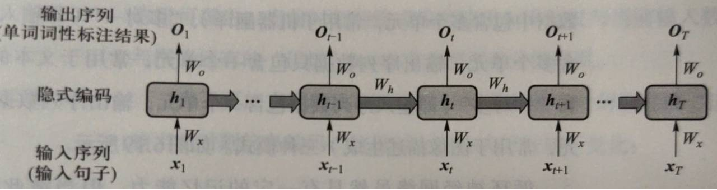
Parameter W_x will x_t maps to implicit encoding__ t, parameter W_o will _ t mapped to predictive output O_t, __ t_1 passes through the parameter W_ _Participate__ Generation of t. W_in Diagram X, W_o and W_ Is a multiplexing parameter.

It can also be understood as follows:

Where S(t-1) from the previous moment participates in the calculation of S(t) from the next moment.

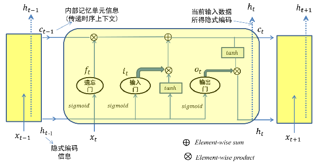
Long-term and short-term memory network LSTM

This section can take a look at the Big Guys video on Station B, and I'll make a summary: lstm principle

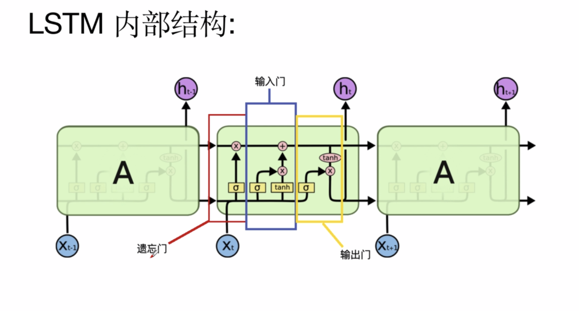
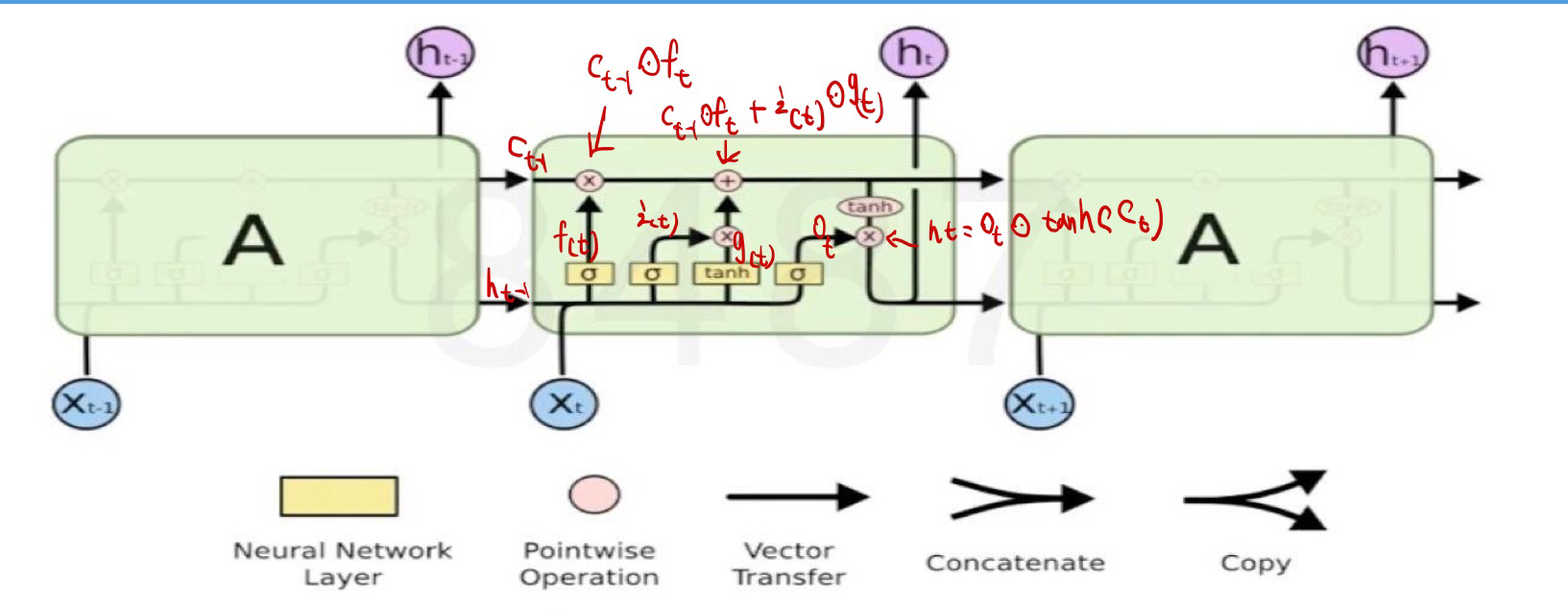
The main purpose of lstm is to understand the calculation of several doors:

Look at the overall formula

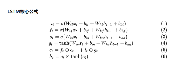
The specific operations are as follows:The first four equations correspond to the results of the following four activation function operations, which multiply the hidden information h(t-1) of the previous step with the information x(t) of the current input, perform the feature fusion operation, then the forgotten weight f(t) is multiplied by the cell information unit C(t-1) of the previous step, and then added by the newly entered feature information i(t) by g(t) (where g(t) The new cell information C(t) is obtained as a feature selection operation, and then the sixth step is performed to get the output of the current hidden state. Then the hidden state result is mapped linearly by a layer, and the classification problem can be implemented by a softmax operation.

On dimension issues:
For example, enter a paragraph: (x_1,..., x_t_1,x_t,x_t+1,..., x_T), x_t-1 can be seen as a word, which in NLP tasks is a vector of words that is usually mapped to (1,512), which is represented here as 1d. The dimensions i(t), f(t), o(t) in lstm are the same as h(t), which can be recorded as 1h, which is set by itself when the lstm module is called. So, in connection with the above formulas, when we train, we are training weight matrix, W(i,i), W(i,f) and so on, which are all dh-dimensional, while W(h,i), W(h,f) and hidden information state operations are h H.

RNN LSTM Handwritten Number Recognition

# 1. Loading datasets
import torch
import torch.nn as nn
import torchvision.transforms as transforms
import torchvision.datasets as datasets
import torchvision
import numpy as np
import pandas as pd
import matplotlib.pyplot as plt



# 6. Define a function: Show a batch of data
def imshow(inp, title=None):
    inp = inp.numpy().transpose((1, 2, 0))
    mean = np.array([0.485, 0.456, 0.406]) # mean value
    std = np.array([0.229, 0.224, 0.225]) # standard deviation
    inp = std * inp + mean
    inp = np.clip(inp, 0, 1) # Limit speed to 0-1
    plt.imshow(inp)
    plt.show()
    if title is not None:
        plt.title(title)
    #plt.pause(1)




# 7. Define RNN model
class RNN_Model(nn.Module):
    def __init__(self, input_dim, hidden_dim, layer_dim, output_dim):
        super(RNN_Model, self).__init__()
        self.hidden_dim = hidden_dim
        self.layer_dim = layer_dim
        self.rnn = nn.RNN(input_dim, hidden_dim, layer_dim, batch_first=True, nonlinearity='relu')
        # Full Connection Layer
        self.fc = nn.Linear(hidden_dim, output_dim)

    def forward(self, x):
        # (layer_dim, batch_size, hidden_dim)
        h0 = torch.zeros(self.layer_dim, x.size(0), self.hidden_dim).requires_grad_().to(device)
        # Separate hidden states to avoid gradient explosion
        out, hn = self.rnn(x, h0.detach())
        out = self.fc(out[:, -1, :])
        return out


# 1. Define the model
class LSTM_Model(nn.Module):
    def __init__(self, input_dim, hidden_dim, layer_dim, output_dim):
        super(LSTM_Model, self).__init__()  # Initialize construction methods in parent class
        self.hidden_dim = hidden_dim
        self.layer_dim = layer_dim
        # Building LSTM Model
        self.lstm = nn.LSTM(input_dim, hidden_dim, layer_dim, batch_first=True)
        # Full Connection Layer
        self.fc = nn.Linear(hidden_dim, output_dim)

    def forward(self, x):
        # Initialization Hidden Layer State is all 0
        # (layer_dim, batch_size, hidden_dim)
        h0 = torch.zeros(self.layer_dim, x.size(0), self.hidden_dim).requires_grad_().to(device)
        # Initialize cell state
        c0 = torch.zeros(self.layer_dim, x.size(0), self.hidden_dim).requires_grad_().to(device)
        # Separate hidden states to avoid gradient explosion
        out, (hn, cn) = self.lstm(x, (h0.detach(), c0.detach()))
        # Only the state of the last hidden layer is required
        out = self.fc(out[:, -1, :])
        return out

def train(train_loader,test_loader,net,Loss_Function,learning_rate,plot_loss,plot_accuary,model_name):
    model=net

    #nn.CrossEntropyLoss()
    # 10. Define Optimizer
    learning_rate = learning_rate

    optimizer = torch.optim.SGD(model.parameters(), lr=learning_rate)
    # 13. Model Training
    sequence_dim = 28  # Sequence Length
    loss_list = []  # Save loss
    accuracy_list = []  # Save accuracy
    iteration_list = []  # Number of Save Loops

    iter = 0
    for epoch in range(EPOCHS):
        for i, (images, labels) in enumerate(train_loader):
            model.train()  # Declaration Training
            # Converting batch data into RNN input dimensions
            images = images.view(-1, sequence_dim, input_dim).requires_grad_().to(device)
            labels = labels.to(device)
            # Gradient Zeroing (otherwise it will continue to accumulate)
            optimizer.zero_grad()
            # Forward propagation
            outputs = model(images)
            # Calculate loss
            loss = Loss_Function(outputs, labels)
            # Reverse Propagation
            loss.backward()
            # Update parameters
            optimizer.step()
            # Counter auto plus 1
            iter += 1
            # Model validation
            if iter % 500 == 0:
                model.eval()  # statement
                # Calculate the accuracy of validation
                correct = 0.0
                total = 0.0
                # Iterate test sets, get data, predict
                for images, labels in test_loader:
                    images = images.view(-1, sequence_dim, input_dim).to(device)
                    # model prediction
                    outputs = model(images)
                    # Obtain subscript for maximum prediction probability
                    predict = torch.max(outputs.data, 1)[1]
                    # Statistical Test Set Size
                    total += labels.size(0)
                    # Statistical Judgment/Forecast Correct Quantity
                    if torch.cuda.is_available():
                        correct += (predict.cuda() == labels.cuda()).sum()
                    else:
                        correct += (predict == labels).sum()
                # Calculation
                accuracy = correct / total * 100
                # Save accuracy, loss, iteration
                loss_list.append(loss.data)
                accuracy_list.append(accuracy)
                iteration_list.append(iter)
                # Print Information
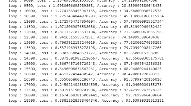
                print("loop : {}, Loss : {}, Accuracy : {}".format(iter, loss.item(), accuracy))
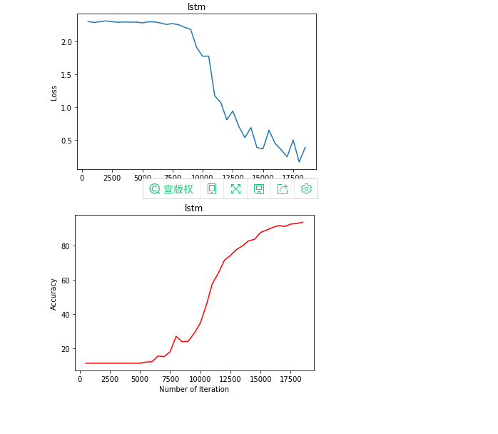
    if plot_loss==True:
        # Visualization loss
        plt.plot(iteration_list, loss_list)
        plt.xlabel('Number of Iteration')
        plt.ylabel('Loss')
        plt.title(model_name)
        plt.show()
    if plot_accuary==True:
        # Visual accuracy
        plt.plot(iteration_list, accuracy_list, color='r')
        plt.xlabel('Number of Iteration')
        plt.ylabel('Accuracy')
        plt.title(model_name)
        plt.savefig('{}_mnist.png'.format(model_name))
        plt.show()


if __name__ == "__main__":
    # 2. Download mnist dataset
    trainsets = datasets.MNIST(root='./data', train=True, download=True, transform=transforms.ToTensor()) # format conversion

    testsets = datasets.MNIST(root='./data', train=False, transform=transforms.ToTensor())


    print(trainsets.data.shape)
    # 4. Define Hyperparameters
    BATCH_SIZE = 32 # Size of data read per batch
    EPOCHS = 10 # Training 10 rounds

    # 5. Create iterative objects for datasets, that is, read data from one batch to one batch
    train_loader = torch.utils.data.DataLoader(dataset=trainsets, batch_size=BATCH_SIZE, shuffle=True)

    test_loader = torch.utils.data.DataLoader(dataset=testsets, batch_size=BATCH_SIZE, shuffle=True)

    # View batch data


    # 8. Initialize the model
    input_dim = 28  # Input Dimension
    hidden_dim = 100  # Hidden Dimension, Neuron
    layer_dim = 2  # 2-Layer RNN
    output_dim = 10  # Output Dimension

    model_rnn = RNN_Model(input_dim, hidden_dim, layer_dim, output_dim)
    model_lstm=LSTM_Model(input_dim, hidden_dim, layer_dim, output_dim)

    # Determine if there is a GPU
    device = torch.device('cuda:0' if torch.cuda.is_available() else 'cpu')
    model_lstm.to(device=device)
    #  Define loss function
    criterion = nn.CrossEntropyLoss()

    train(train_loader,test_loader,model_lstm,criterion,learning_rate=0.01,plot_loss=True,plot_accuary=True,model_name="lstm")