Content introduction

This paper introduces cluster analysis with a simple example of Python using Keans for cluster analysis.

Cluster analysis or clustering is the task of grouping a group of objects, Make objects in the same group (called clusters) more similar (in a sense) to objects in other groups (clusters) It is the main task of exploratory data mining and the common technology of statistical data analysis. It is used in many fields, including machine learning, pattern recognition, image analysis, information retrieval, bioinformatics, data compression and computer graphics.

General application scenarios

• Group classification of target users: cluster the target groups according to the variables selected for operation or business purposes, divide the target groups into several subdivided groups with obvious characteristics, and adopt refined and personalized operations and services for these subdivided groups in operation activities to improve operation efficiency and business effect.
• Value combination of different products: cluster many product categories according to specific index variables. Subdivide the product system into multi-dimensional product combinations with different values, different purposes, and formulate corresponding product development plans, operation plans and service plans on this basis.
• Explore and discover outliers and outliers: mainly risk control applications. There may be a risk component of fraud at the outlier.

Common methods of clustering

It is divided into algorithms based on partition, hierarchy, density, grid, statistics, model, etc. typical algorithms include K-means (classical clustering algorithm), DBSCAN, two-step clustering, BIRCH, spectral clustering, etc.

Implementation of Keans clustering

import numpy as np
import matplotlib.pyplot as plt
from sklearn.cluster import KMeans
from sklearn import metrics
import random

# Randomly generate 100 groups of data containing 3 groups of characteristics
feature = [[random.random(),random.random(),random.random()] for i in range(100)]
label = [int(random.randint(0,2)) for i in range(100)]

# Convert data format
x_feature = np.array(feature)

# Training clustering model
n_clusters = 3  # Set the number of clusters
model_kmeans = KMeans(n_clusters=n_clusters, random_state=0)  # Establish clustering model object
model_kmeans.fit(x_feature)  # Training clustering model
y_pre = model_kmeans.predict(x_feature)  # Predictive clustering model
y_pre

Evaluation index of clustering

inertias is the attribute of the K-means model object, which represents the sum of the cluster centers closest to the sample. It is used as an unsupervised evaluation index without the label of real classification results. The smaller the value, the better. The smaller the value, the more concentrated the distribution of samples among classes, that is, the smaller the distance within classes.

# The sum of the nearest cluster centers
inertias = model_kmeans.inertia_  

adjusted_rand_s: The Adjusted Rand Index calculates the similarity measure between the two clusters by considering all sample pairs and count pairs allocated in the same or different clusters in the predicted and real clusters. The Adjusted Rand Index obtains a value close to 0 independent of the sample size and category through the adjustment of the RAND index, and its value range is [- 1, 1], negative numbers represent bad results. The closer to 1, the better, which means that the clustering results are more consistent with the real situation.

# Adjusted Rand index
adjusted_rand_s = metrics.adjusted_rand_score(label, y_pre)  

mutual_info_s: Mutual information (MI) is the amount of information about another random variable contained in one random variable. Here, it refers to the measure of similarity between two labels of the same data, and the result is a non negative value.

# Mutual information
mutual_info_s = metrics.mutual_info_score(label, y_pre) 

adjusted_mutual_info_s: Adjusted mutual information (AMI). The adjusted mutual information is the adjustment score of the mutual information score. It takes into account that for clusters with a larger number, the MI is usually higher, regardless of whether there is actually more information sharing. It corrects this effect by adjusting the probability of clustering clusters. When two cluster sets are the same (i.e. exact match), the return value of AMI is 1; the average expected AMI of random partition (independent label) is about 0, or it may be negative.

# Adjusted mutual information
adjusted_mutual_info_s = metrics.adjusted_mutual_info_score(label, y_pre)  

homogeneity_s: Homogeneity: if all clusters only contain data points belonging to members of a single class, the clustering results will meet the homogeneity. The larger the value range [0,1] means that the clustering results are more consistent with the real situation.

# Homogenization score
homogeneity_s = metrics.homogeneity_score(label, y_pre)  

completeness_s: Integrity score: if all data points as members of a given class are elements of the same cluster, the clustering result meets the integrity. Its value range is [0,1]. The larger the value, the more consistent the clustering result is with the real situation.

# Integrity score
completeness_s = metrics.completeness_score(label, y_pre)  

v_measure_s: It is the harmonic average value between homogenization and integrity, v = 2 (uniformity integrity) / (uniformity + integrity). Its value range is [0,1]. The larger the value, the more consistent the clustering results are with the real situation.

v_measure_s = metrics.v_measure_score(label, y_pre)  

silhouette_s: The contour coefficient (Silhouette) is used to calculate the average contour coefficient of all samples. It is calculated by using the average intra cluster distance and the average nearest cluster distance of each sample. It is an unsupervised evaluation index. Its highest value is 1, and the lowest value is - 1,0. Values near 0 represent overlapping clusters, and negative values usually indicate that samples have been assigned to the wrong cluster.

# Average contour coefficient
silhouette_s = metrics.silhouette_score(x_feature, y_pre, metric='euclidean')  

calinski_harabaz_s: The score is defined as the ratio of intra cluster dispersion to inter cluster dispersion, which is an unsupervised evaluation index.

# Calinski and Harabaz score
calinski_harabaz_s = metrics.calinski_harabasz_score(x_feature, y_pre)  

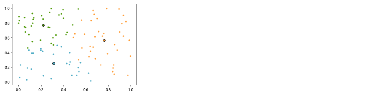
Visualization of clustering effect

# Model effect visualization
centers = model_kmeans.cluster_centers_  # Centers by category
colors = ['#4EACC5', '#FF9C34', '#4E9A06']  # Set colors for different categories
plt.figure()  # Create canvas
for i in range(n_clusters):  # Cyclic read category
    index_sets = np.where(y_pre == i)  # Found an index collection of the same class
    cluster = x_feature[index_sets]  # The data of the same class is divided into a cluster subset
    plt.scatter(cluster[:, 0], cluster[:, 1], c=colors[i], marker='.')  # Show the sample points in the cluster subset
    plt.plot(centers[i][0], centers[i][1], 'o', markerfacecolor=colors[i], markeredgecolor='k',
             markersize=6)  # Show the center of each cluster subset
plt.show()  # Display image

Data prediction

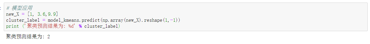
# Model application
new_X = [1, 3.6,9.9]
cluster_label = model_kmeans.predict(np.array(new_X).reshape(1,-1))
print ('The cluster prediction result is: %d' % cluster_label)