tushare financial data interface package
- pip install tushare
- Function: provide relevant specified financial data
- Related documents: Tushare - financial data interface package
Demand: stock analysis
Use the tushare package to obtain the historical quotation data of a stock.
- tushare financial data interface package, based on which historical trading data of any stock can be obtained
- pip install tushare
data processing
Use the tushare package to obtain the historical quotation data of a stock
df = ts.get_k_data(code='600519',start='2010-01-10')
Persistent storage of DF df.to_xxx()
#Store df's data locally
df.to_csv('./maotai.csv')
Load external data pd.read_xxx()
#Load external data into df: read_xxx()
df=pd.read_csv('./maotai.csv')
print(df.head())
Output results
   Unnamed: 0        date     open    close     high      low    volume    code
0           5  2010-01-11  104.400  102.926  105.230  102.422  24461.03  600519
1           6  2010-01-12  103.028  105.708  106.040  102.492  31063.40  600519
2           7  2010-01-13  104.649  103.022  105.389  102.741  37924.44  600519
3           8  2010-01-14  103.379  107.552  107.974  103.379  46454.64  600519
4           9  2010-01-15  107.533  108.401  110.641  107.533  45938.50  600519
Delete Unnamed: 0 column
In the drop series of functions
- axis=0 represents the row and 1 represents the column
- inplace=True will delete the original data directly
#Delete Unnamed: 0 column
df.drop(labels="Unnamed: 0",axis=1,inplace=True)  #inplace=True means that the original column is deleted and not saved
print(df.head())
Output result: Unnamed: 0 is no longer available
         date     open    close     high      low    volume    code
0  2010-01-11  104.400  102.926  105.230  102.422  24461.03  600519
1  2010-01-12  103.028  105.708  106.040  102.492  31063.40  600519
2  2010-01-13  104.649  103.022  105.389  102.741  37924.44  600519
3  2010-01-14  103.379  107.552  107.974  103.379  46454.64  600519
4  2010-01-15  107.533  108.401  110.641  107.533  45938.50  600519
Converts the time of the string type of the date column to the time series type
#Converts the time of the string type of the date column to the time series type
df["date"]=pd.to_datetime(df["date"])
print(df["date"].dtype)
Output result: the date column has become a time type
datetime64[ns]
Use the date column as the row index of the source data
#Use the date column as the row index of the source data
df.set_index("date",inplace=True)
print(df.head())
Output result: the time column is used as the row index
              open    close     high      low    volume    code
date
2010-01-11  104.400  102.926  105.230  102.422  24461.03  600519
2010-01-12  103.028  105.708  106.040  102.492  31063.40  600519
2010-01-13  104.649  103.022  105.389  102.741  37924.44  600519
2010-01-14  103.379  107.552  107.974  103.379  46454.64  600519
2010-01-15  107.533  108.401  110.641  107.533  45938.50  600519
Data analysis
1. Output all the dates when the closing price of the stock is more than 3% higher than the opening price.
(closing opening) / opening > 0.03
print((df['close']-df['open'])/df['open']>0.03)
Output results
date
2010-01-11    False
2010-01-12    False
2010-01-13    False
2010-01-14     True
2010-01-15    False
              ...
2021-11-16    False
Experience: in df related operations, once the Boolean value is returned, the next step is to take the Boolean value as the row index of the original data
Obtain the line data meeting the demand (the closing price is more than 3% higher than the opening price)
# It is found that the Boolean value can be used as the row index of df, and the row data corresponding to true can be directly extracted
df2=df.loc[(df['close'] - df['open']) / df['open'] > 0.03]
print(df2.head())
Output result: only true rows are reserved
date
2010-01-14  103.379  107.552  107.974  103.379  46454.64  600519
2010-01-28  104.566  107.974  108.708  104.336  30267.52  600519
2010-04-21   91.573   94.458   94.579   90.431  63365.87  600519
2010-05-07   80.406   82.965   83.195   80.087  31254.76  600519
2010-05-21   82.576   85.645   85.894   81.982  27341.38  600519

Process finished with exit code 0
Get the date when the requirement is met
#Get the date when the requirement is met
print(df2.index)
Output results
DatetimeIndex(['2010-01-14', '2010-01-28', '2010-04-21', '2010-05-07',
               '2010-05-21', '2010-08-02', '2010-08-30', '2010-10-20',
               '2010-11-10', '2010-11-23',
               ...
               '2021-05-25', '2021-07-28', '2021-08-02', '2021-08-10',
               '2021-08-24', '2021-09-01', '2021-09-17', '2021-09-24',
               '2021-09-27', '2021-10-13'],
              dtype='datetime64[ns]', name='date', length=172, freq=None)

Process finished with exit code 0
2. The date when the opening price of the stock is more than 2% lower than the closing price of the previous day.
- (opening closing the day before) / closing the day before < -0.02
- shift(n) You can move the column n rows as a whole. A positive number means moving down and a negative number means moving up
- df['close'].shift(1) represents the closing number of the previous day
#The date when the opening price of the stock is more than 2% lower than the closing price of the previous day
df3=df.loc[(df['open'] - df['close'].shift(1))/ df['close'].shift(1)<- 0.02].index
print(df3)
Output results
DatetimeIndex(['2010-04-26', '2010-04-30', '2011-08-05', '2012-03-27',
               '2012-08-10', '2012-11-22', '2012-12-04', '2012-12-24',
               '2013-01-16', '2013-01-25', '2013-09-02', '2014-04-25',
               '2015-01-19', '2015-05-25', '2015-07-03', '2015-07-08',
               '2015-07-13', '2015-08-24', '2015-09-02', '2015-09-15',
               '2017-11-17', '2018-02-06', '2018-02-09', '2018-03-23',
               '2018-03-28', '2018-07-11', '2018-10-11', '2018-10-24',
               '2018-10-25', '2018-10-29', '2018-10-30', '2019-05-06',
               '2019-05-08', '2019-10-16', '2020-01-02', '2020-02-03',
               '2020-03-13', '2020-03-23', '2020-10-26', '2021-02-26',
               '2021-03-04', '2021-04-28', '2021-08-20', '2021-11-01'],
              dtype='datetime64[ns]', name='date', freq=None)

Process finished with exit code 0
3. If I buy one hand (100 stocks) on the first trading day of each month and sell all stocks on the last trading day of each year from January 1, 2010, how is my income so far?
- Buy stock
- On the first trading day of each month, buy primary stocks according to the opening price
- A complete year requires 12 purchases of 1200 stocks in 12 hands (100 stocks in one hand)
- Sell stock
- All stocks are sold on the last trading day of each year according to the opening price (12-31)
- A full year needs to sell 1200 shares
- Note: in 2020, this person can only buy 700 stocks and cannot sell them. However, when calculating the total return, the value of the remaining shares needs to be included
- How to calculate the remaining stock value:
- 700 * opening price on the buying day
- How to calculate the remaining stock value:
Take the data from 2010 to 2020
#Take the data from 2010 to 2020
new_df=df["2010":"2020"] #If the row index is time series data, the index value can be obtained in this way
print(new_df)
Output results
              open     close      high       low    volume    code
date
2010-01-11   104.400   102.926   105.230   102.422  24461.03  600519
2010-01-12   103.028   105.708   106.040   102.492  31063.40  600519
2010-01-13   104.649   103.022   105.389   102.741  37924.44  600519
2010-01-14   103.379   107.552   107.974   103.379  46454.64  600519
2010-01-15   107.533   108.401   110.641   107.533  45938.50  600519
...              ...       ...       ...       ...       ...     ...
2020-12-25  1802.990  1830.000  1847.000  1800.000  23088.00  600519
2020-12-28  1826.600  1873.000  1888.800  1826.050  30080.00  600519
2020-12-29  1873.000  1867.000  1886.800  1855.000  22868.00  600519
2020-12-30  1870.000  1933.000  1933.000  1869.990  34452.00  600519
2020-12-31  1941.000  1998.000  1998.980  1939.000  38860.00  600519

[2663 rows x 6 columns]

Process finished with exit code 0
resample of data
- M represents the month and is output on the last day of each month
# Take out and group all the monthly data from 2010 to 2020, and take out the first data of each month
df_monthly=new_df.resample(rule="M").first()
print(df_monthly)
Output results
#The following figure shows some data examples. date actually shows the first trading day of each month, which is caused by its internal bug
               open     close      high       low    volume    code
date
2010-01-31   104.400   102.926   105.230   102.422  24461.03  600519
2010-02-28   107.769   107.776   108.216   106.576  29655.94  600519
2010-03-31   106.219   106.085   106.857   105.925  21734.74  600519
2010-04-30   101.324   102.141   102.422   101.311  23980.83  600519
2010-05-31    81.676    82.091    82.678    80.974  23975.16  600519
...              ...       ...       ...       ...       ...     ...
2020-08-31  1686.880  1668.000  1696.580  1660.000  34661.00  600519
2020-09-30  1792.000  1801.980  1802.000  1775.010  31640.00  600519
2020-10-31  1692.000  1696.000  1706.420  1688.000  34240.00  600519
2020-11-30  1675.000  1674.010  1695.000  1672.000  21066.00  600519
2020-12-31  1726.000  1737.000  1738.990  1720.010  28196.00  600519

[132 rows x 6 columns]

Process finished with exit code 0
Calculate the total cost of buying stocks
#Calculate the total cost of buying stocks
cost=df_monthly["open"].sum()*100
print(cost)
resample of data
- A represents the year, and the last data of 2020 is removed
# All the annual data from 2010 to 2020 are taken out and grouped, and the last data of each year is taken out
df_yearly=new_df.resample(rule="A").last()[0:-1] # Remove the last data in 2020
print(df_yearly)
Output results
               open     close      high       low   volume    code
date
2010-12-31   117.103   118.469   118.701   116.620  46084.0  600519
2011-12-31   138.039   138.468   139.600   136.105  29460.0  600519
2012-12-31   155.208   152.087   156.292   150.144  51914.0  600519
2013-12-31    93.188    96.480    97.179    92.061  57546.0  600519
2014-12-31   157.642   161.056   161.379   157.132  46269.0  600519
2015-12-31   207.487   207.458   208.704   207.106  19673.0  600519
2016-12-31   317.239   324.563   325.670   317.239  34687.0  600519
2017-12-31   707.948   687.725   716.329   681.918  76038.0  600519
2018-12-31   563.300   590.010   596.400   560.000  63678.0  600519
2019-12-31  1183.000  1183.000  1188.000  1176.510  22588.0  600519

Process finished with exit code 0
How much is the income from selling stocks
#How much is the income from selling stocks
income=df_yearly['open'].sum()*1200
print("The total return on shares sold on the last day of each year is:{}".format(income))
Output results
The total return on shares sold on the last day of each year is 4368184.8
Calculate the value of the remaining shares
#Calculate the value of the remaining shares
last=df['open'][-1]*700
print("2020 The proceeds from the sale of the remaining shares in the year are:{}".format(last))
Output results
2020 The proceeds from the sale of the remaining shares in the year were 1294300.0
Calculate total income + last - cost
#Calculate total revenue
print(income + last - cost)
The total code of the above 2 questions
# -*-coding:utf-8-*-
import pandas as pd
import tushare as ts
df = ts.get_k_data(code='600519',start='2010-01-10')
print(df.head())
#Store df's data locally
df.to_csv('./maotai.csv')
#Load external data into df: read_xxx()
df=pd.read_csv('./maotai.csv')
print(df.head())
#Delete Unnamed: 0 column
df.drop(labels="Unnamed: 0",axis=1,inplace=True)
print(df.head())
#Converts the time of the string type of the date column to the time series type
df["date"]=pd.to_datetime(df["date"])
print(df["date"].dtype)
#Use the date column as the row index of the source data
df.set_index("date",inplace=True)
print(df.head())
#Output all the dates when the closing price of the stock is more than 3% higher than the opening price
print((df['close']-df['open'])/df['open']>0.03)
# It is found that the Boolean value can be used as the row index of df, and the row data corresponding to true can be directly extracted
df2=df.loc[(df['close'] - df['open']) / df['open'] > 0.03]
print(df2.head())
#Get the date when the requirement is met
print(df2.index)
#The date when the opening price of the stock is more than 2% lower than the closing price of the previous day
df3=df.loc[(df['open'] - df['close'].shift(1))/ df['close'].shift(1)<- 0.02].index
print(df3)
#Take the data from 2010 to 2020
new_df=df["2010":"2020"] #If the row index is time series data, the index value can be obtained in this way
print(new_df)
# Take out and group all the monthly data from 2010 to 2020, and take out the first data of each month
df_monthly=new_df.resample(rule="M").first()
print(df_monthly)
#Calculate the total cost of buying stocks
cost=df_monthly["open"].sum()*100
print(cost)
# All the annual data from 2010 to 2020 are taken out and grouped, and the last data of each year is taken out
df_yearly=new_df.resample(rule="A").last()[0:-1] # Remove the last data in 2020
print(df_yearly)
#How much is the income from selling stocks
income=df_yearly['open'].sum()*1200
print("The total return on shares sold on the last day of each year is:{}".format(income))
#Calculate the value of the remaining shares
last=df['open'][-1]*700
print("2020 The proceeds from the sale of the remaining shares in the year are:{}".format(last))
#Calculate total revenue
print(income + last - cost)
Demand: Double average strategy formulation
get data
- Use the tushare package to obtain the historical quotation data of a stock
- Calculate the 5-day moving average and 30 day moving average of the stock's historical data
- What is the moving average?
- For each trading day, you can calculate the moving average of the previous N days, and then connect these moving average values to form a line, which is called the N-day moving average. The common moving average line has indicators of 5 days, 10 days, 30 days, 60 days, 120 days and 240 days.
- 5-day and 10-day are the reference indicators for short-term operation, which are called daily moving average indicators;
- 30 day and 60 day are medium-term moving average indicators, called quarterly moving average indicators;
- The 120 day and 240 day are long-term moving average indicators, which are called annual moving average indicators.
- For each trading day, you can calculate the moving average of the previous N days, and then connect these moving average values to form a line, which is called the N-day moving average. The common moving average line has indicators of 5 days, 10 days, 30 days, 60 days, 120 days and 240 days.
- Calculation method of moving average: MA = (C1+C2+C3+...+Cn)/N C: closing price of a day n: moving average period (days)
- What is the moving average?
# -*-coding:utf-8-*-
import  pandas as pd
import  numpy as np
import  matplotlib.pyplot as plt
from pandas import  Series,DataFrame
import  tushare as ts

df=ts.get_k_data(code='600519',start='1999-01-10') # get data
df.to_csv('./maotai2.csv') # Store data
df=pd.read_csv('./maotai2.csv')  #Read data
df.drop(labels='Unnamed: 0',axis=1,inplace=True)  #Delete Unnamed: 0 column
df['date']=pd.to_datetime(df['date']) # Time from string to time
df.set_index('date',inplace=True)  # Set date as index
print(df.head())
Calculate and develop a double moving average
rolling(5) gets the first five data of each data and counts itself
Average()
The first few data show NaN because there is not enough data in front of it
# -*-coding:utf-8-*-
import  pandas as pd
import  numpy as np
import  matplotlib.pyplot as plt
from pandas import  Series,DataFrame
import  tushare as ts

df=ts.get_k_data(code='600519',start='1999-01-10') # get data
df.to_csv('./maotai2.csv') # Store data
df=pd.read_csv('./maotai2.csv')  #Read data
df.drop(labels='Unnamed: 0',axis=1,inplace=True)  #Delete Unnamed: 0 column
df['date']=pd.to_datetime(df['date']) # Time from string to time
df.set_index('date',inplace=True)  # Set date as index
print(df.head())

#Calculate and develop a double moving average
df=df['2010':'2020']
ma5=df['close'].rolling(5).mean()  #5-day moving average
ma30=df['close'].rolling(30).mean()  #30 day moving average

#mapping
plt.figure(figsize=(15,8),dpi=80)
plt.plot(ma5[50:200],linewidth=3,label="ma5")
plt.plot(ma30[50:200],linewidth=3,label="ma30")
plt.legend() #Set legend style
plt.show()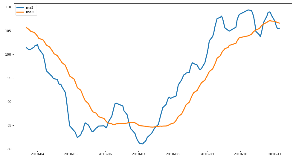
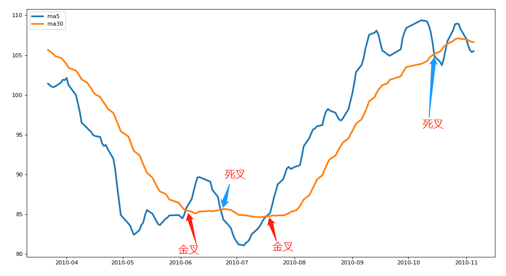
Analyze and output all golden cross dates and dead cross dates
Golden fork and dead fork in stock analysis technology
The golden fork and dead fork in stock analysis technology can be simply explained as follows:
- There are two lines in the analysis index, one is the index line in a short time, and the other is the index line in a long time.
- If the indicator line turns upward for a short time and crosses the indicator line for a long time, this state is called "golden fork";
- If the indicator line turns downward for a short time and crosses the indicator line for a long time, this state is called "dead fork";
- In general, after the occurrence of gold fork, the operation tends to buy; Dead forks tend to sell. Of course, golden fork and dead fork are only one of the analysis indicators. They should be used together with many other indicators to increase the accuracy of operation.
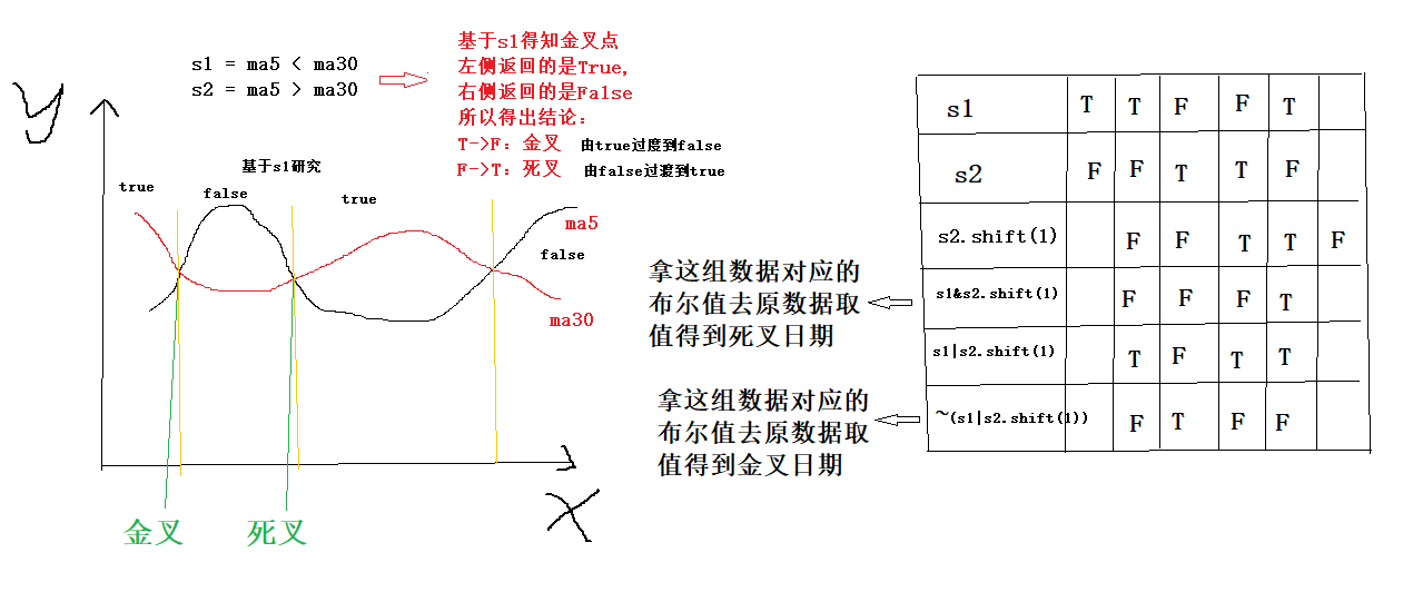
s1=ma5<ma30 kdj
s2=ma5>ma30 Dead fork
s1 and s2 are Boolean values
Data analysis
If I start from January 1, 2010, the initial capital is 100000 yuan, the golden fork tries to buy, and the dead fork sells all, what is my stock speculation yield so far?
- analysis:
- The unit price for buying and selling stocks shall be the opening price
- Timing of buying and selling stocks
- In the end, there will be surplus stocks that have not been sold
- There will be. If the last day is a golden fork, buy stocks. Estimate the value of the remaining shares and calculate the total income.
- The unit price of the remaining shares is the closing price on the last day.
- There will be. If the last day is a golden fork, buy stocks. Estimate the value of the remaining shares and calculate the total income.
Find out all the golden cross and dead cross dates of the time node
Analyze and output all golden cross dates and dead cross dates
s1=ma5<ma30
print(s1)
s2=ma5>ma30
print(s2)
death_date=df.loc[s1&s2.shift(1)].index
print(death_date)
gold_date=df.loc[~(s1|s2.shift(1))].index
print(gold_date)
Output results
DatetimeIndex(['2010-02-26', '2010-06-23', '2010-10-15', '2010-11-02',
               '2010-12-24', '2011-03-02', '2011-03-30', '2011-09-08',
               '2011-12-08', '2012-07-24', '2012-08-02', '2012-08-15',
               '2012-09-21', '2012-11-07', '2012-12-25', '2013-01-18',
               '2013-03-18', '2013-06-21', '2013-07-12', '2013-10-25',
               '2013-11-26', '2013-12-04', '2014-04-01', '2014-04-30',
               '2014-08-22', '2014-09-16', '2014-10-13', '2014-11-21',
               '2015-01-19', '2015-06-17', '2015-07-17', '2015-09-28',
               '2015-11-26', '2015-12-10', '2016-01-05', '2016-08-05',
               '2016-08-18', '2016-11-21', '2017-07-06', '2017-09-08',
               '2017-11-29', '2018-02-05', '2018-03-27', '2018-06-28',
               '2018-07-23', '2018-07-31', '2018-10-15', '2018-12-25',
               '2019-05-10', '2019-07-19', '2019-11-28', '2020-01-03',
               '2020-02-28', '2020-03-18', '2020-08-10', '2020-09-21',
               '2020-10-27'],
              dtype='datetime64[ns]', name='date', freq=None)
DatetimeIndex(['2010-01-04', '2010-01-05', '2010-01-06', '2010-01-07',
               '2010-01-08', '2010-01-11', '2010-01-12', '2010-01-13',
               '2010-01-14', '2010-01-15', '2010-01-18', '2010-01-19',
               '2010-01-20', '2010-01-21', '2010-01-22', '2010-01-25',
               '2010-01-26', '2010-01-27', '2010-01-28', '2010-01-29',
               '2010-02-01', '2010-02-02', '2010-02-03', '2010-02-04',
               '2010-02-05', '2010-02-08', '2010-02-09', '2010-02-10',
               '2010-02-11', '2010-02-12', '2010-06-04', '2010-07-19',
               '2010-10-22', '2010-11-10', '2011-02-11', '2011-03-14',
               '2011-04-28', '2011-10-25', '2012-02-10', '2012-07-25',
               '2012-08-09', '2012-09-12', '2012-09-27', '2012-12-21',
               '2013-01-10', '2013-03-12', '2013-04-17', '2013-07-03',
               '2013-10-22', '2013-11-11', '2013-11-28', '2014-01-23',
               '2014-04-03', '2014-06-23', '2014-09-04', '2014-09-29',
               '2014-11-20', '2014-11-28', '2015-02-13', '2015-07-15',
               '2015-09-16', '2015-10-09', '2015-12-03', '2015-12-21',
               '2016-02-22', '2016-08-11', '2016-10-13', '2016-11-25',
               '2017-07-24', '2017-09-18', '2017-12-15', '2018-03-16',
               '2018-05-09', '2018-07-18', '2018-07-25', '2018-09-20',
               '2018-12-04', '2019-01-03', '2019-06-14', '2019-08-13',
               '2020-01-02', '2020-02-19', '2020-03-03', '2020-04-02',
               '2020-08-19', '2020-10-14', '2020-11-05'],
              dtype='datetime64[ns]', name='date', freq=None)

Process finished with exit code 0
Store the golden cross date and the dead cross date into two Series respectively, take the date as the index of the Series, and take 0 and 1 as the value of the Series
- The date corresponding to value 1 is the golden fork date
- The date corresponding to value 0 is a dead cross date
series_1 = Series(data=1, index=gold_date)
#print(series_1)
series_2 = Series(data=0, index=death_date)
#print(series_2)
# Cascade the golden cross and dead cross dates and sort them in ascending order according to the time index
# Remove the data of the first 30 items, because these dates have continuous golden or dead cross dates
series_all=series_1.append(series_2).sort_index()[30:]
print(series_all)
Income calculation
- The golden fork shall buy as much as possible, and all the dead forks shall be sold. The unit price of buying and selling stocks shall use the opening price
- Special situation: yesterday was the golden fork. You can only buy but not sell. If you have any remaining stocks, you also need to calculate their value into the total income
#Income calculation
first_money = 100000 # Principal (immutable)
cost_money = 100000 # (variable)
hold = 0 # Number of shares held
for index in series_all.index:
    # Index is series_ Display index of all
    if series_all[index] == 1:  # The day is a golden fork, and you need to buy stocks
        # Find out the unit price of the stock
        price = df['open'][index]
        # Try to buy as many shares as you can with all your money
        hand = cost_money // (price * 100)
        hold = hand * 100  # How many stocks have you bought
        # The money spent on buying stocks from cost_money minus
        cost_money -= (hold * price)
    else:  # Sell stock
        # Find the unit price of selling shares
        price = df['open'][index]
        cost_money += (price * hold)
        hold = 0

# Calculate the actual value of the remaining shares (how to know if there are any remaining shares)
last_money = hold * df['open'][-1]
# Total revenue
print(last_money + cost_money - first_money)
Output result: 2203311.1