When it comes to data mining machine learning, the myth about beer diapers has long been heard in my impression. This problem often appears in articles related to data warehouses, which shows how far and deep the beer diaper problem has impacted the field of data mining.Look first at the cause: The story of beer and diapers originated in Wal-Mart supermarkets in the United States in the 1990s. Wal-Mart supermarket managers analyzed sales data and found an incomprehensible phenomenon: in some specific cases, beer and diaper were two seemingly unrelated goods.This unique sales phenomenon, often found in the same shopping basket, attracts the attention of managers who, according to follow-up surveys, find it in young fathers who often take a bottle of beer home with them while buying diapers.
While enjoying this issue, not everyone will be concerned about its implementation details.The beer diaper problem belongs to association analysis, where hidden relationships between items are found from a set of data sets and is a typical unsupervised learning.The itemset of association rules can be isomorphic such as beer->diaper or isomeric such as summer->air conditioning stock.
The Apriori algorithm in this article is mainly based on the association analysis of frequent sets, which is also one of the ten classical data mining algorithms. By default, the association analysis in this article refers to the association analysis based on frequent sets.
Below are descriptions of the Apriori algorithm that are collected by individuals to aid in memory. If misleading, please correct.
A collection of items is called an itemset.An item set containing K items is called a k-item set.
Item set I is represented as {i1,i2,...ik-1,ik}, I can be beer, diaper, milk, and so on.
Set D represents the training set, which corresponds to multiple transactions (which can be understood as shopping tickets) and each transaction corresponds to a subset of I (different goods).
Candidate set, a set of items constructed by association combinations.Candidate sets are pruned to form frequent itemsets.
Frequent itemsets are those that meet the minimum support criteria, and all subsets of them must be frequent, understood as a group of goods that often appear together in the same basket.
Support formula: support = P(A and B), since the total number of training set transactions is relatively fixed, it can be simplified to the frequency of A and B (denominator same can be ignored).
The Apriori algorithm has a very important property, that is, a priori property, which means that all subsets of frequent itemsets must also be frequent.In general, the irony of this nature is used in the implementation of the algorithm, that is, if an itemset is not a frequent itemset, its superitemset must not be a frequent itemset.This property can greatly reduce the number of times the algorithm traverses the data.
The two K itemsets (frequent sets) need to be joined to generate a super itemset (candidate set) if both have the same K-1 item or if K is the initial frequent set.
Maximum frequent itemset, the final frequent itemset that satisfies the minimum support condition.
Association rules are represented as A->B, where A and B are subsets of I, and the intersection of A and B is empty. Rule correlation is unidirectional, so it can be interpreted as a cause-and-effect relationship.
The association rule deduced from the calculated set of K terms should satisfy the confidence level condition and be interpreted as larger than the set probability value.
Confidence formula: confidence = P(A)|P(A and B) = support(A and B)/support(A)
From the description above, we can see that the concept of candidate set, frequent set and subset appears many times in this algorithm. How to construct and manipulate the set is the key of Apriori algorithm, and the language that is best at set operation is SQL.Also based on this series, Thinking
in SQL, see how to use SQL to reproduce the classic beer diaper sales myth.
Unlike the exhaustion method, according to the nature of frequent sets, the Aprior algorithm uses a layer-by-layer search method, which consists of the following five steps:
1. First, the candidate set (K-1) is initialized according to set D, and then the K-1 frequent set is obtained according to the minimum support condition.
2.K-1 frequent sets self-join to obtain K candidate sets.The first K-1 frequent set is constructed in step 1, while the other rounds are obtained in step 3 (the frequent set is pruned from the candidate set).
3. Trim the candidate set.How do I prune?If the support of the candidate set is less than the minimum support, it will be pruned; in addition, subsets of the candidate set that are not frequent will be pruned (this is a more complex process).
4. Recursive step 2, 3, the algorithm terminates with the following condition: if the frequency set from the connection is no longer frequent, take the last frequent set as the result.
5. Build candidate association rules and prune with minimum confidence to form final Association rules.
Now that I have a better understanding of this algorithm, I need to start to implement it, and give a brief explanation of my ideas:
1. Build and import training sets for machine learning
2. Create collection types to facilitate SQL interaction with PLSQL
3. Create a support calculation function for output itemset support
4. Create a function that builds a very large frequent set (recursively generates a frequent set, and pruning depends on the support function of step 3)
5. The principal queries the SQL, uses the functions created in step 4 to build association rules, and prunes the output based on the minimum confidence level
The steps are as follows (personal environment ORACLE XE 11.2):
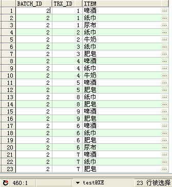
1. Build training set D, create table DM_APRIORI_LEARNING_T to store training set
CREATE TABLE DM_APRIORI_LEARNING_T
(
BATCH_ID NUMBER ,--batch ID,Distinguish training sets D
TRX_ID NUMBER ,--Transactional Notes ID
ITEM VARCHAR2(100) --commodity
) ;
2. Create collection types so that SQL can interact with PLSQL.Each itemset may have a different number of items belonging to an itemset ID.
CREATE OR REPLACE TYPE DM_APRIORI_SET_OBJ IS OBJECT (
GID NUMBER ,--Itemset ID
ITEM VARCHAR2(100),--term
SUPPORT NUMBER --Support
);
CREATE OR REPLACE TYPE DM_APRIORI_SET_TAB IS TABLE OF DM_APRIORI_SET_OBJ;
3. Create a function for itemset support calculation, return a set of itemset support, rely on APRIORI training set table, where P_BATCH_ID is used to define the training set, P_TAB is used to pass in the candidate set, focus on how to judge the itemset can be fully matched by the training set and the number of matches SQL implementation, need to be set-oriented thinking, that is, Thinking in SQL.
CREATE OR REPLACE FUNCTION FUN_DM_APRIORI_SUPPORT(P_BATCH_ID NUMBER,
                                                  P_TAB      DM_APRIORI_SET_TAB,
                                                  P_DEBUG    NUMBER DEFAULT 0)
  RETURN DM_APRIORI_SET_TAB IS
  RTAB DM_APRIORI_SET_TAB; --Result Frequent Set
BEGIN
  WITH TA AS
   (SELECT A.GID, A.ITEM, COUNT(1) OVER(PARTITION BY A.GID) KCNT --Number of items per group
      FROM TABLE(P_TAB) A --candidate set
    ),
  TB2 AS
   ( --Match facts to calculate support
    SELECT A.GID,
            A.ITEM,
            A.KCNT,
            T.TRX_ID GID2,
            COUNT(1) OVER(PARTITION BY A.GID, T.TRX_ID) MATCH_CNT --Number of matching transactions per group
      FROM TA A
      JOIN DM_APRIORI_LEARNING_T T
        ON A.ITEM = T.ITEM
       AND T.BATCH_ID = P_BATCH_ID) --Calculate Itemset GID Frequency of simultaneous occurrences in the training set SUPPORT
  SELECT DM_APRIORI_SET_OBJ(GID, NULL, COUNT(1) / KCNT) --Calculate support
         BULK COLLECT
    INTO RTAB
    FROM TB2
   WHERE MATCH_CNT = KCNT --The number of items matches the number of transaction matches before they are all matched
   GROUP BY GID, KCNT;

  RETURN RTAB;
END;
4. Create a recursive function to construct a superset of K-item frequent sets, recursively construct a very frequent set of items according to the specified parameters, and here you can specify the maximum K value of P_MAXLVL to limit the recursive level (default is unlimited). Focus on the SQL implementation of frequent set connections to construct candidate supersets, which is the core part of the algorithm.G in SQL, block ROW BY ROW loop processing ideas, note that you might get lost if you don't have collection-oriented thinking.
CREATE OR REPLACE FUNCTION FUN_DM_APRIORI_FREQ_SET --Apriori Association rule pruning
(P_BATCH_ID NUMBER, --batch
 P_TAB      DM_APRIORI_SET_TAB, --Frequent set of previous rounds
 P_CURK     NUMBER, --Before Constructing Frequent Sets K Original value
 P_SUPPORT  NUMBER, --Minimum Support
 P_MAXLVL   NUMBER DEFAULT NULL --Maximum Recursion Level, Maximum K value
 ) RETURN DM_APRIORI_SET_TAB IS
  ATAB DM_APRIORI_SET_TAB; --Frequency of the previous round K-1 Itemset
  RTAB DM_APRIORI_SET_TAB; --Frequent construction generation K Itemset
BEGIN
  --Initialization ATAB
  IF P_CURK = 1 THEN
    SELECT DM_APRIORI_SET_OBJ(ROWNUM, ITEM, SUPPORT)
      BULK COLLECT INTO ATAB
      FROM (SELECT ITEM, COUNT(1) SUPPORT
              FROM DM_APRIORI_LEARNING_T
             WHERE BATCH_ID = P_BATCH_ID
             GROUP BY ITEM
            HAVING COUNT(1) >= P_SUPPORT);
    IF P_MAXLVL = 1 THEN
      RETURN ATAB;
    END IF;
  ELSE
    ATAB := P_TAB;
  END IF;
  WITH TA AS
   (SELECT * FROM TABLE(ATAB)),
  TB0 AS
   ( --K=1 Temporal Constructions K+1 Itemset
    SELECT RANK() OVER(ORDER BY A.GID, B.GID) GID, A.ITEM ITEM1, B.ITEM ITEM2
      FROM TA A
      JOIN TA B
        ON A.ITEM < B.ITEM
       AND P_CURK = 1 --Note this conditional switch
    ),
  TB AS
   ( --K>1 Temporal Constructions K+1 Itemset
    SELECT RANK() OVER(ORDER BY GID1, GID2) GID, GID1, GID2, ITEM
      FROM (SELECT A.GID GID1,
                    B.GID GID2,
                    A.ITEM,
                    COUNT(1) OVER(PARTITION BY A.GID, B.GID) MATCH_CNT
               FROM TA A
               JOIN TA B
                 ON A.ITEM = B.ITEM
                AND A.GID < B.GID)
     WHERE P_CURK > 1
       AND MATCH_CNT = P_CURK - 1 --Itemset join condition: K-1 Items are the same
    ),
  TC AS
   ( --Candidate Set Construction
    SELECT DISTINCT C.GID, A.ITEM --Non-first round candidate set construction
      FROM TB C
      JOIN TA A
        ON (C.GID1 = A.GID OR C.GID2 = A.GID)
       AND A.ITEM NOT IN (SELECT K.ITEM FROM TB K WHERE K.GID = C.GID)
    UNION ALL
    SELECT GID, ITEM
      FROM TB
    UNION ALL --K=1 subsection
    SELECT GID, ITEM --Initial candidate set
      FROM TB0 UNPIVOT(ITEM FOR COL IN(ITEM1, ITEM2))),
  TE AS
   (SELECT GID,
           ITEM,
           LISTAGG(ITEM) WITHIN GROUP(ORDER BY ITEM) OVER(PARTITION BY GID) VLIST --Itemset LIST,Easy to calculate
      FROM TC),
  TF AS
   ( --K+1 Itemset
    SELECT ROWNUM RNUM, GID, ITEM
      FROM TE A
     WHERE GID = (SELECT MIN(GID) FROM TE B WHERE A.VLIST = B.VLIST)),
  --The following is a calculation of all K Is the set subset all frequent
  TG AS
   ( --K+1=>K Set Subset  C(K+1,K)= C(K+1,1)
    SELECT A.RNUM, A.GID, B.ITEM
      FROM TF A
      JOIN TF B
        ON A.GID = B.GID
       AND A.ITEM != B.ITEM),
  TH AS
   (SELECT G.RNUM, G.GID, COUNT(1) OVER(PARTITION BY G.GID) CNT2 --Match in each group K Number of terms of degree
      FROM TG G
      JOIN TA A --TA Is a known set of frequent items
        ON G.ITEM = A.ITEM
     GROUP BY G.RNUM, G.GID, A.GID
    HAVING COUNT(1) = P_CURK --K Set elements need to be matched individually K second
    ),
  TI AS
   (SELECT * FROM TH WHERE CNT2 = P_CURK + 1 --Leave Frequent Itemsets
    ),
  TKC AS
   ( --Candidate Set (all subsets frequent)
    SELECT TF.GID, TF.ITEM
      FROM TF
      JOIN TI
        ON TF.RNUM = TI.RNUM
       AND TF.GID = TI.GID),
  TKCA AS
   ( --Constructing candidate subset parameters
    SELECT CAST(MULTISET (SELECT GID, ITEM, NULL FROM TKC) AS
                 DM_APRIORI_SET_TAB) STAB
      FROM DUAL),
  TK2 AS
   ( --Support for pruning filtration
    SELECT TKC.*, TS2.SUPPORT
      FROM TKCA
     CROSS JOIN TABLE(FUN_DM_APRIORI_SUPPORT(P_BATCH_ID, TKCA.STAB)) TS2 --Candidate subset support
      JOIN TKC
        ON TKC.GID = TS2.GID
       AND TS2.SUPPORT >= P_SUPPORT)
  SELECT DM_APRIORI_SET_OBJ(GID, ITEM, SUPPORT) BULK COLLECT
    INTO RTAB
    FROM TK2;
  IF P_MAXLVL = P_CURK + 1 THEN
    RETURN RTAB; --Satisfy Maximum Item
  ELSIF RTAB.COUNT = 0 THEN
    RETURN ATAB; --Itemset is empty, take previous itemset
  ELSE
    --Recursive Itemset
    RETURN FUN_DM_APRIORI_FREQ_SET(P_BATCH_ID,
                                   RTAB,
                                   P_CURK + 1,
                                   P_SUPPORT,
                                   P_MAXLVL);
  END IF;
END;
Once the function is created, you can make a few simple queries to help understand:
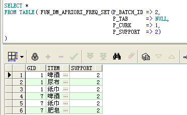
A. When you query the results of a calculation of a very large and frequent itemset, you can see that there are two or three itemsets of the result
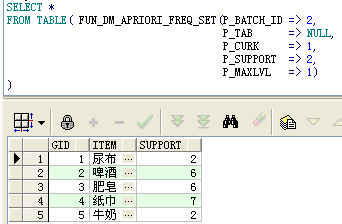
b. Query the initial itemset, specifying a maximum search level of 1, resulting in 6 1 itemsets
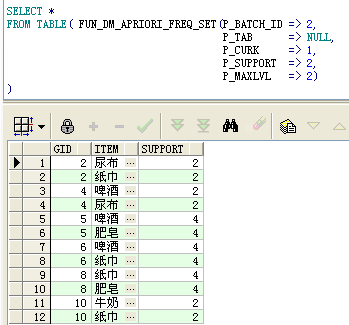
c. Query frequent 2 itemsets, specifying a maximum search level of 2, resulting in 6 2 itemsets
d. Query the support level corresponding to the two frequent itemsets, note the use of CAST and MULTISET, do not explain
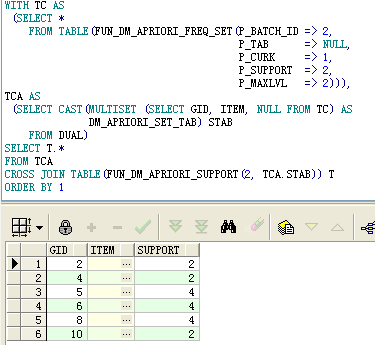
5. The main body queries the SQL, uses the functions created in steps 3 and 4 to build association rules, prunes the output results according to the minimum confidence level, and uses the parameter set PARAMS (support level 2, confidence level 60%) to drive the whole disk, Thinking in SQL, all at once, as follows:
WITH PARAMS AS
 (SELECT 2 BATCH_ID, 2 SUPPORT, 0.6 CONF FROM DUAL),
TA AS
 ( --Frequent Sets
  SELECT GID, ITEM, SUPPORT, COUNT(1) OVER(PARTITION BY GID) KCNT --Number of Items of Set
    FROM PARAMS P
   CROSS JOIN TABLE(FUN_DM_APRIORI_FREQ_SET(P.BATCH_ID, NULL, 1, P.SUPPORT))),
TB AS
 ( --k Subset preparation of sets
  SELECT ROWNUM GID,
          TA.GID OGID,
          TA.ITEM,
          TA.KCNT,
          TA.SUPPORT KSUPPORT,
          LEVEL LVL,
          '{' || LTRIM(SYS_CONNECT_BY_PATH(ITEM, ','), ',') || '}' ITEM_LIST --Itemset description for rule output
    FROM TA
  CONNECT BY LEVEL <= KCNT - 1
         AND PRIOR ITEM < ITEM
         AND PRIOR GID = GID),
TC AS
 ( --k A subset of sets
  SELECT A.GID, A.OGID, A.ITEM_LIST, A.KCNT, A.LVL, B.ITEM
    FROM TB A
    JOIN TB B
      ON A.OGID = B.OGID
     AND B.LVL <= A.LVL
     AND B.GID = (SELECT MAX(C.GID)
                    FROM TB C
                   WHERE C.OGID = B.OGID
                     AND C.LVL = B.LVL
                     AND C.GID <= A.GID)),
TCA AS --Assembly Set Parameters
 (SELECT BATCH_ID,
         SUPPORT,
         CONF,
         CAST(MULTISET (SELECT GID, ITEM, NULL FROM TC) AS
              DM_APRIORI_SET_TAB) STAB
    FROM PARAMS),
TD AS
 ( --Subset support calculation
  SELECT A.GID,
          B.OGID,
          B.KCNT,
          B.KSUPPORT,
          B.LVL,
          B.ITEM_LIST,
          A.SUPPORT,
          TCA.CONF
    FROM TCA
   CROSS JOIN TABLE(FUN_DM_APRIORI_SUPPORT(TCA.BATCH_ID, TCA.STAB)) A
    JOIN TB B
      ON A.GID = B.GID),
TE AS
 (SELECT A.GID AGID,
         A.OGID,
         A.ITEM_LIST AITEM_LIST,
         A.KSUPPORT,
         A.SUPPORT,
         B.GID BGID,
         B.ITEM_LIST BITEM_LIST,
         A.CONF,
         A.KSUPPORT / A.SUPPORT REAL_CONF --Confidence Result
    FROM TD A
    JOIN TD B
      ON A.OGID = B.OGID
     AND A.LVL + B.LVL = A.KCNT --a and b Elements belonging to a very frequent set
     AND NOT EXISTS ( --a hand over b Is empty
          SELECT ITEM
            FROM TC
           WHERE GID = A.GID
          INTERSECT
          SELECT ITEM FROM TC WHERE GID = B.GID))
SELECT AITEM_LIST || '->' || BITEM_LIST RULE_DESC, REAL_CONF
  FROM TE
 WHERE REAL_CONF >= CONF --Confidence of pruning filter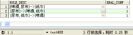
Classic algorithms like beer diapers allow us to expand our thinking, not just in the vertical direction (specializing in technology, limited self-esteem), otherwise we will fall into the trap of "too academic".Instead of focusing solely on basket analysis, brainstorming your lateral thinking extensions can reveal many scenarios.For example, as a DBA developer, you often analyze questions such as which tables are frequently queried simultaneously by associations, which columns appear in predicates at the same time, and how to create composite indexes, redundant acceleration columns, and redundant acceleration tables can have a strategic impact on overall system performance.The training set can be formed by mining and analyzing the SQL of production library regularly. The related itemsets between tables, the related itemsets of predicate columns and the related rules can be found by manipulating the frequent set. The support weight can also be given by combining Euler's theorem.This will provide effective decision-making basis for efficient database design and operation.Of course, real-world development can't make people think too much about strategic technical elements, and performance requirements are just a temporary pleasure.So while many of the ideas that you've worked for N years are only partially grounded.Agile + result-oriented will inevitably lead to guerrilla warfare mentality (rules of association derived personally) that many people will agree with.
Back to the topic, the SQL language has inherent advantages in data processing. Thinking in SQL, a set-oriented thinking engine, processes data through relational operations (and, intersect, multiply, divide), and ORACLE's efficient SQL engine is responsible for circular processing.Combined with advanced ORACLE development techniques, ORACLE databases can also customize machine learning capabilities by continually summarizing and generalizing and injecting soul algorithms.