
House price forecasting is an introductory competition on kaggle. Generally speaking, it gives you 79 features about house price, and then predicts house price according to the characteristics. The evaluation index of housing price forecast is root mean square error (RMSE), that is: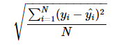
1. Data Exploratory Analysis
First read the data using pandas module
import pandas as pd

train = pd.read_csv("train.csv")
test = pd.read_csv("test.csv")
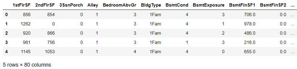
Display the first few rows of training set and test set respectively
train.head()
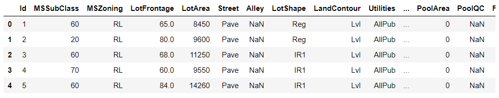
test.head()
There are discrete and continuous values in the above feature data, and there are a lot of missing values. Because of the large number of features, we only visualize the housing price data based on the year of construction.
import matplotlib.pyplot as plt
import seaborn as sns

plt.figure(figsize=(10,8))
sns.boxplot(train.YearBuilt, train.SalePrice)
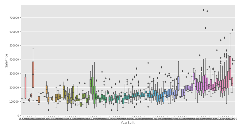
From the year of construction alone, the general trend is that old houses are cheaper and new ones are more expensive.
2. Data cleaning
Abnormal Point Processing
Firstly, we observe whether there is a linear relationship based on the housing area visualization data.
plt.figure(figsize=(12,6))
plt.scatter(x=train.GrLivArea, y=train.SalePrice)##It can be used to observe linear relationships.
plt.xlabel("GrLivArea", fontsize=13)
plt.ylabel("SalePrice", fontsize=13)
plt.ylim(0,800000)
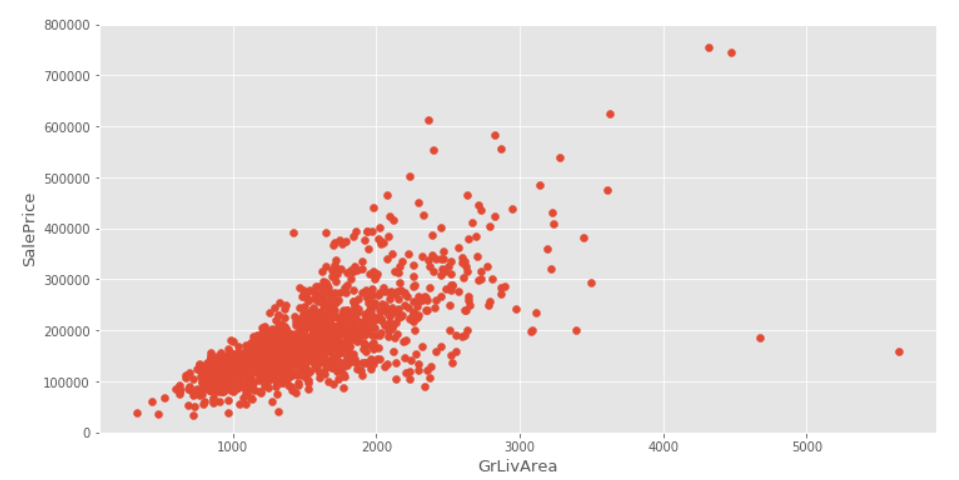
From the scatter plot above, we can see that the larger the area of the house, the higher the house price, but there are two abnormal points in the lower right corner of the picture which violate this linear relationship and need to be removed.
# Remove data with GrLivArea > 4000 and SalePrice < 300000
train.drop(train[(train["GrLivArea"]>4000)&(train["SalePrice"]<300000)].index,inplace=True)
data processing
For convenience, the training set and test set data are processed together.
full = pd.concat([train,test],ignore_index=True)
First remove the Id column, which is useless for prediction.
full.drop("Id",axis=1,inplace=True)
print(full.shape)  # (2917, 80)
There are 2917 samples including the training set test set. Each sample actually contains 79 features. Since the training set data contains the final housing price data, 80 samples are shown here.
Null Value Filling and Deleting
As we said before, there are many missing values in the sample. We need to deal with the missing values. First, we look at the missing values of those features and sort the number of missing values from low to high.
miss = full.isnull().sum() #Statistical Number of Null Values
miss[miss>0].sort_values(ascending=True)#Rank from low to high
GarageArea         1
SaleType           1
KitchenQual        1
BsmtFinSF1         1
BsmtFinSF2         1
GarageCars         1
TotalBsmtSF        1
Exterior2nd        1
Exterior1st        1
BsmtUnfSF          1
Electrical         1
Functional         2
Utilities          2
BsmtHalfBath       2
BsmtFullBath       2
MSZoning           4
MasVnrArea        23
MasVnrType        24
BsmtFinType1      79
BsmtFinType2      80
BsmtQual          81
BsmtCond          82
BsmtExposure      82
GarageType       157
GarageYrBlt      159
GarageFinish     159
GarageCond       159
GarageQual       159
LotFrontage      486
FireplaceQu     1420
SalePrice       1459
Fence           2346
Alley           2719
MiscFeature     2812
PoolQC          2908
dtype: int64
Because eigenvalues contain character and numeric types, they need to be processed separately.
None is used to fill in the following character types:
cols1 = ["PoolQC" , "MiscFeature", "Alley", "Fence", "FireplaceQu", "GarageQual", "GarageCond", "GarageFinish", "GarageYrBlt", "GarageType", "BsmtExposure", "BsmtCond", "BsmtQual", "BsmtFinType2", "BsmtFinType1", "MasVnrType"]
for col in cols1:
    full[col].fillna("None",inplace=True)
The following numerical type features are filled with 0:
cols=["MasVnrArea", "BsmtUnfSF", "TotalBsmtSF", "GarageCars", "BsmtFinSF2", "BsmtFinSF1", "GarageArea"]
for col in cols:
    full[col].fillna(0, inplace=True)
Fill in the null value of lotfrontage (using the mean of this column)
full["LotFrontage"].fillna(np.mean(full["LotFrontage"]),inplace=True)
Modal filling of the following columns
cols2 = ["MSZoning", "BsmtFullBath", "BsmtHalfBath", "Utilities", "Functional", "Electrical", "KitchenQual", "SaleType","Exterior1st", "Exterior2nd"]
for col in cols2:
    full[col].fillna(full[col].mode()[0], inplace=True)
Next, look at what hasn't been filled in, and find that only test data has no label (house price) column.
full.isnull().sum()[full.isnull().sum()>0] # So far we've filled in the null values.
SalePrice    1459
dtype: int64
3. Data Preprocessing - Converting Character Type to Numeric Type
Converting some digital features into category features. It is best to use LabelEncoder and get_dummies to implement these functions.
from sklearn.preprocessing import LabelEncoder #Label coding

lab = LabelEncoder()
Label encoding of the following features
full["Alley"] = lab.fit_transform(full.Alley)
full["PoolQC"] = lab.fit_transform(full.PoolQC)
full["MiscFeature"] = lab.fit_transform(full.MiscFeature)
full["Fence"] = lab.fit_transform(full.Fence)
full["FireplaceQu"] = lab.fit_transform(full.FireplaceQu)
full["GarageQual"] = lab.fit_transform(full.GarageQual)
full["GarageCond"] = lab.fit_transform(full.GarageCond)
full["GarageFinish"] = lab.fit_transform(full.GarageFinish)
full["GarageYrBlt"] = lab.fit_transform(full.GarageYrBlt)
full["GarageType"] = lab.fit_transform(full.GarageType)
full["BsmtExposure"] = lab.fit_transform(full.BsmtExposure)
full["BsmtCond"] = lab.fit_transform(full.BsmtCond)
full["BsmtQual"] = lab.fit_transform(full.BsmtQual)
full["BsmtFinType2"] = lab.fit_transform(full.BsmtFinType2)
full["BsmtFinType1"] = lab.fit_transform(full.BsmtFinType1)
full["MasVnrType"] = lab.fit_transform(full.MasVnrType)
full["BsmtFinType1"] = lab.fit_transform(full.BsmtFinType1)

full["MSZoning"] = lab.fit_transform(full.MSZoning)
full["BsmtFullBath"] = lab.fit_transform(full.BsmtFullBath)
full["BsmtHalfBath"] = lab.fit_transform(full.BsmtHalfBath)
full["Utilities"] = lab.fit_transform(full.Utilities)
full["Functional"] = lab.fit_transform(full.Functional)
full["Electrical"] = lab.fit_transform(full.Electrical)
full["KitchenQual"] = lab.fit_transform(full.KitchenQual)
full["SaleType"] = lab.fit_transform(full.SaleType)
full["Exterior1st"] = lab.fit_transform(full.Exterior1st)
full["Exterior2nd"] = lab.fit_transform(full.Exterior2nd)
In this way, most of the features are converted to numerical types.
full.head()
Finally, delete the column corresponding to the house price
full.drop("SalePrice",axis=1,inplace=True) #delete
full.shape  # (2917, 79)
4. pipeline Construction - pipeline
Facilitate the combination of various features and the processing of features, and facilitate the subsequent feature redo of machine learning.
Firstly, the transformation function is constructed:
from sklearn.base import BaseEstimator, TransformerMixin
from sklearn.pipeline import Pipeline, make_pipeline #Building pipelines
from scipy.stats import skew #skewness


class labelenc(BaseEstimator, TransformerMixin):
    def __init__(self):
        pass

    def fit(self,X,y=None):
        return self
    ##Make a label code for three years, here you can add it yourself.
    def transform(self,X):
        lab=LabelEncoder()
        X["YearBuilt"] = lab.fit_transform(X["YearBuilt"])
        X["YearRemodAdd"] = lab.fit_transform(X["YearRemodAdd"])
        X["GarageYrBlt"] = lab.fit_transform(X["GarageYrBlt"])
        X["BldgType"] = lab.fit_transform(X["BldgType"])

        return X

class skew_dummies(BaseEstimator, TransformerMixin):
    def __init__(self,skew=0.5):#skewness
        self.skew = skew

    def fit(self,X,y=None):
        return self

    def transform(self,X):
        #Removing the object data types, most of them are numeric.
        X_numeric=X.select_dtypes(exclude=["object"])
        #Anonymous functions, in the form of dictionaries
        skewness = X_numeric.apply(lambda x: skew(x))
        #Conditions are used to select skew >= 0.5 index, and all data are retrieved to prevent data loss.
        skewness_features = skewness[abs(skewness) >= self.skew].index
        #Find logarithm to make it more normal distribution
        X[skewness_features] = np.log1p(X[skewness_features])
        ##One-click solitary heat, solitary heat coding
        X = pd.get_dummies(X)
        return X
Building pipelines
pipe = Pipeline([##Meaning of Pipeline Construction
    ('labenc', labelenc()),
    ('skew_dummies', skew_dummies(skew=2)),
    ])
Pipeline processing of data
full2 = full.copy()
pipeline_data = pipe.fit_transform(full2)
pipeline_data.shape  # (2917, 178)
Re-dividing the processed data into training set and test set
n_train=train.shape[0] # Number of rows in training set
X = pipeline_data[:n_train] # Remove the training set after processing
test_X = pipeline_data[n_train:] # Data after n_train is taken out as test set
y= train.SalePrice
X_scaled = StandardScaler().fit(X).transform(X) # Do transformation
y_log = np.log(train.SalePrice) # log is used here, which is more in line with normal distribution.
#Get the test set
test_X_scaled = StandardScaler().fit_transform(test_X)
5. Feature Selection - Selection Based on Feature Importance
Feature selection of training set using algorithm
from sklearn.linear_model import Lasso

lasso=Lasso(alpha=0.001)
lasso.fit(X_scaled,y_log)

FI_lasso = pd.DataFrame({"Feature Importance":lasso.coef_}, index=pipeline_data.columns)

FI_lasso.sort_values("Feature Importance",ascending=False)#Sort from high to low
FI_lasso[FI_lasso["Feature Importance"]!=0].sort_values("Feature Importance").plot(kind="barh",figsize=(15,25))
plt.xticks(rotation=90)
plt.show()##Drawing display
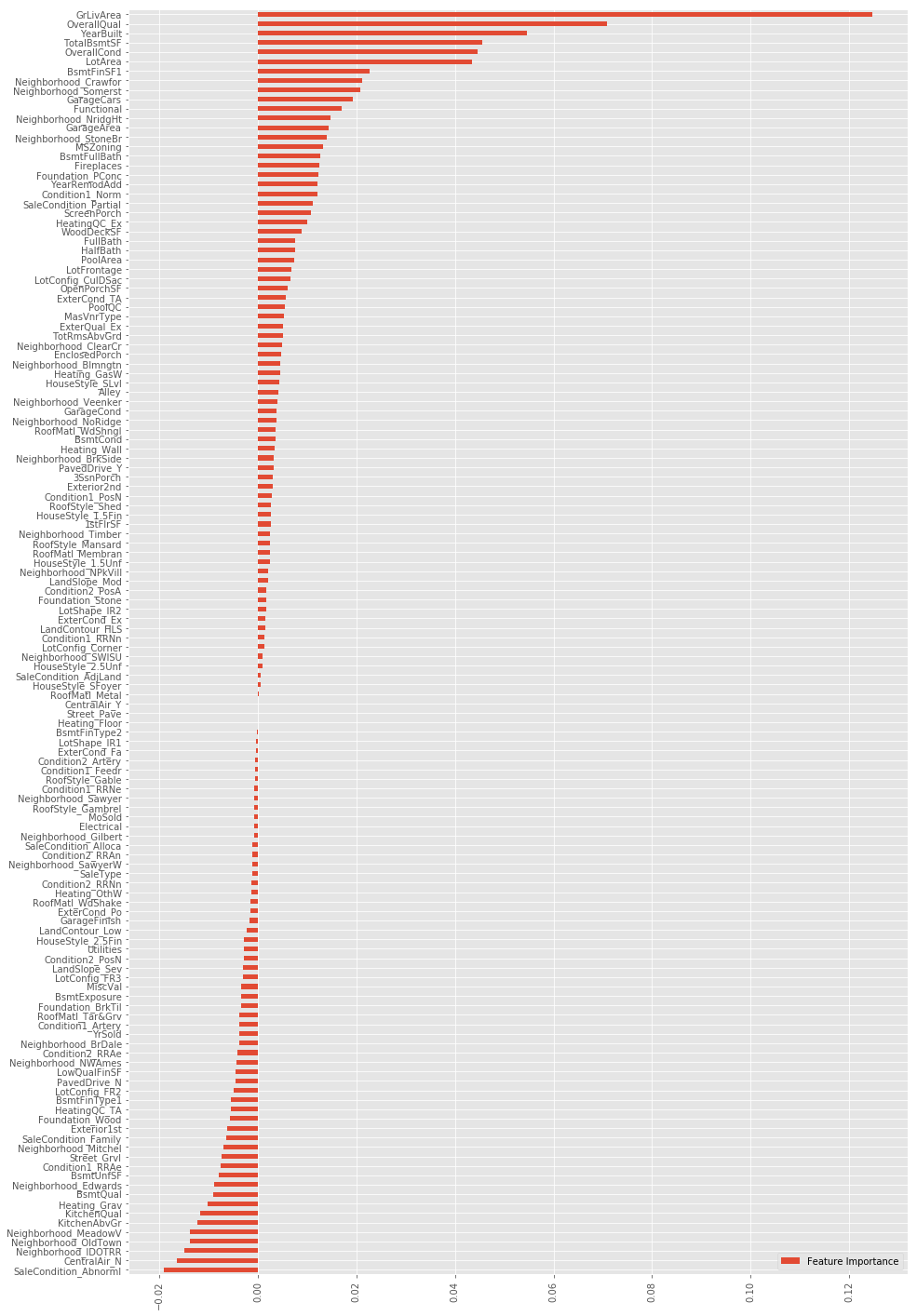
After obtaining the feature importance map, feature selection and redo can be carried out.
class add_feature(BaseEstimator, TransformerMixin):#Define your own transformation function -- fit_transform is defined by yourself
    def __init__(self,additional=1):
        self.additional = additional

    def fit(self,X,y=None):
        return self

    def transform(self,X):
        if self.additional==1:
            X["TotalHouse"] = X["TotalBsmtSF"] + X["1stFlrSF"] + X["2ndFlrSF"]
            X["TotalArea"] = X["TotalBsmtSF"] + X["1stFlrSF"] + X["2ndFlrSF"] + X["GarageArea"]

        else:
            X["TotalHouse"] = X["TotalBsmtSF"] + X["1stFlrSF"] + X["2ndFlrSF"]
            X["TotalArea"] = X["TotalBsmtSF"] + X["1stFlrSF"] + X["2ndFlrSF"] + X["GarageArea"]

            X["+_TotalHouse_OverallQual"] = X["TotalHouse"] * X["OverallQual"]
            X["+_GrLivArea_OverallQual"] = X["GrLivArea"] * X["OverallQual"]
            X["+_oMSZoning_TotalHouse"] = X["MSZoning"] * X["TotalHouse"]
            X["+_oMSZoning_OverallQual"] = X["MSZoning"] + X["OverallQual"]
            X["+_oMSZoning_YearBuilt"] = X["MSZoning"] + X["YearBuilt"]
            X["+_oNeighborhood_TotalHouse"] = X["Neighborhood"] * X["TotalHouse"]
            X["+_oNeighborhood_OverallQual"] = X["Neighborhood"] + X["OverallQual"]
            X["+_oNeighborhood_YearBuilt"] = X["Neighborhood"] + X["YearBuilt"]
            X["+_BsmtFinSF1_OverallQual"] = X["BsmtFinSF1"] * X["OverallQual"]

            X["-_oFunctional_TotalHouse"] = X["Functional"] * X["TotalHouse"]
            X["-_oFunctional_OverallQual"] = X["Functional"] + X["OverallQual"]
            X["-_LotArea_OverallQual"] = X["LotArea"] * X["OverallQual"]
            X["-_TotalHouse_LotArea"] = X["TotalHouse"] + X["LotArea"]
            X["-_oCondition1_TotalHouse"] = X["Condition1"] * X["TotalHouse"]
            X["-_oCondition1_OverallQual"] = X["Condition1"] + X["OverallQual"]


            X["Bsmt"] = X["BsmtFinSF1"] + X["BsmtFinSF2"] + X["BsmtUnfSF"]
            X["Rooms"] = X["FullBath"]+X["TotRmsAbvGrd"]
            X["PorchArea"] = X["OpenPorchSF"]+X["EnclosedPorch"]+X["3SsnPorch"]+X["ScreenPorch"]
            X["TotalPlace"] = X["TotalBsmtSF"] + X["1stFlrSF"] + X["2ndFlrSF"] + X["GarageArea"] + X["OpenPorchSF"]+X["EnclosedPorch"]+X["3SsnPorch"]+X["ScreenPorch"]


            return X
Add all feature processing to the pipeline
pipe = Pipeline([
    ('labenc', labelenc()),
    ('add_feature', add_feature(additional=2)),
    ('skew_dummies', skew_dummies(skew=4)),
    ])

full3 = full.copy()
pipeline_data = pipe.fit_transform(full3)
pipeline_data.shape  # (2917, 159)

n_train=train.shape[0]#Number of rows in training set
X = pipeline_data[:n_train]#Remove the training set after processing
test_X = pipeline_data[n_train:]#Data after n_train is taken out as test set
y= train.SalePrice
X_scaled = StandardScaler().fit(X).transform(X)#Do transformation
y_log = np.log(train.SalePrice)##What we should pay attention to here is that it is more in line with the normal distribution.
#Get the test set
test_X_scaled = StandardScaler().fit_transform(test_X)
6. Building Decision Tree Model
from sklearn.tree import DecisionTreeRegressor#Import model

model = DecisionTreeRegressor()
model1 =model.fit(X_scaled,y_log)

predict = np.exp(model1.predict(test_X_scaled)) #np.exp is the inverse transformation after the logarithmic transformation above.
result=pd.DataFrame({'Id':test.Id, 'SalePrice':predict})
result.to_csv("submission.csv",index=False)
Upload the resulting submission.csv with a score of about 0.19760