What is a jump watch

The full name of jump list is jump list. It allows you to quickly query, insert and delete a data linked list of ordered and continuous elements. The average search and insertion time complexity of the jump list is O(logn). Fast query is performed by maintaining a multi-level linked list, and the elements in each layer of the linked list are a subset of the elements in the previous layer of the linked list (see the diagram on the right). At the beginning, the algorithm searches in the most sparse level until the element to be found is between two adjacent elements in that level. At this time, the algorithm will jump to the next level and repeat the previous search until the element to be found is found.

A schematic diagram of a jump list. Each box with an arrow represents a pointer, and each row is a linked list of sparse subsequences; The number box at the bottom (yellow) represents an ordered data sequence. The search proceeds down from the most sparse subsequence at the top until the element to be searched is between two adjacent elements of the layer.

Evolution of jump table

For a single linked list, even if the data is ordered, if you want to query one of the data, you can only traverse the linked list from scratch. This is very inefficient and time complexity is very high, which is O(n).
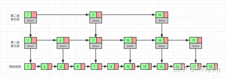
Is there any way to improve the efficiency of query? We can create an "index" for the linked list, which will make the search faster. As shown in the figure below, we extract a node from every two nodes on the basis of the original linked list to establish an index. We call the extracted node the index layer or index, and down represents the pointer to the original linked list node.

Now, if we want to find a data, such as 15, we first traverse the index layer. When we traverse the node with the value of 14 in the index layer, we find that the value of the next node is 17, so the 15 we are looking for must be between the two nodes. At this time, we return to the original linked list through the down pointer of 14 nodes, and then continue to traverse. At this time, we only need to traverse two more nodes to find the data we want. OK, let's look at it from the beginning. In the whole process, we traverse a total of 7 nodes to find the value we want. If we use the original linked list instead of establishing the index layer, we need to traverse 10 nodes.

Through this example, we can see that by establishing an index layer, we need to traverse less times to find a base point, that is, the query efficiency is improved.

So what if we add another index to the index layer? Will there be fewer nodes to traverse and higher efficiency? Let's just try.

Now let's find 15 again. We start from the second level index and finally find 15. We traverse a total of 6 nodes, which is more efficient.

Of course, because the amount of data in our example is very small, the efficiency improvement is not particularly obvious. If we build more layers of indexes when the amount of data is very large, the efficiency improvement will be very obvious. Those who are interested can try it by themselves. We won't give an example here.

This mechanism of adding multi-level indexes to the linked list is the skip list.

How fast does the meter jump

Through the above example, we know that the query efficiency of jump table is higher than that of linked list. How much higher is it? Let's have a look.

To measure the efficiency of an algorithm, we can use time complexity. Here we also use time complexity to compare linked lists and jump lists. As we have said before, the time complexity of the linked list query is O(n). What about the skip list?

If a linked list has n nodes, if one node is extracted from every two nodes to establish an index, the number of nodes of the first level index is about n/2, the number of nodes of the second level index is about n/4, and so on. The number of nodes of the M-level index is about n/(2^m).

If there are M-level indexes, and the number of nodes in level M is two, we can get n/(2^m)=2 through the law we found above, so as to obtain m=log(n)-1. If the original linked list is added, the height of the whole hop list is log(n). When we query the hop table, if each layer needs to traverse K nodes, the final time complexity is O(k*log(n)).

What is the value of K? According to the case that we extract one base point from every two nodes to establish an index, we need to traverse two nodes at most at each level, so k=2. Why does each layer traverse at most two nodes?

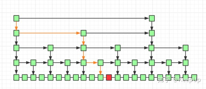
Because we extract a node from every two nodes to establish an index, and the highest level index has only two nodes, and then the next level index adds a node between the two nodes than the previous level index, that is, the median value of the two nodes of the previous level index. Do you think of the binary search we talked about earlier, Each time we just need to judge whether the value to be found is between the current node and the next node.

As shown in the figure above, we need to query the red node. The route we query is the path query indicated by the yellow line. Each level can traverse up to two nodes.

Therefore, the time complexity of querying arbitrary data in the skip table is O(2*log(n)), and the preceding constant 2 can be ignored, which is O(log(n)).

Jump table is to trade space for time

The efficiency of the jump table is higher than that of the linked list, but the jump table needs to store additional multi-level indexes, so it needs more memory space.

It is not difficult to analyze the spatial complexity of the jump table. If a linked list has n nodes, if one node is extracted from every two nodes to establish an index, the number of nodes of the first level index is about n/2, and the number of nodes of the second level index is about n/4. By analogy, the number of nodes of the M-level index is about n/(2^m). We can see that this is an equal ratio sequence.

The node sum of these indexes is n/2+n/4+n/8... + 8+4+2=n-2, so the spatial complexity of the jump table is o(n).

So is there any way to reduce the memory space occupied by indexes? Yes, we can extract an index every three nodes or no five nodes. In this way, the number of index nodes is reduced and the space occupied is less.

Insertion and deletion of skip table

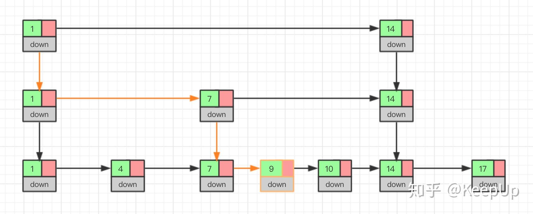
If we want to insert or delete data for the jump table, we first need to find the insertion or deletion location, and then perform the insertion or deletion operation. As we have already known, the time complexity of the jump table query is O(logn), because the time complexity of the insertion and deletion after finding the location is very low, which is O(1), so the time complexity of the final insertion and deletion is also O(longn).

Look at the insertion process through the figure.

If this node also appears in the index, we should delete not only the nodes in the original linked list, but also the nodes in the index. Because the deletion operation in the single linked list needs to get the precursor node of the node to be deleted, and then complete the deletion through pointer operation. Therefore, when looking for the node to be deleted, we must obtain the precursor node. Of course, if we use a two-way linked list, we don't need to consider this problem.

If we keep inserting elements into the jump table, there may be too many nodes between the two index points. If there are too many nodes, our advantage of establishing index will be lost. Therefore, we need to maintain the size balance between the index and the original linked list, that is, when the number of nodes increases, the index increases accordingly, so as to avoid too many nodes between the two indexes and reduce the search efficiency.

The jump table maintains this balance through a random function. When we insert data into the jump table, we can choose to insert the data into the index at the same time. What level of index do we insert? This requires a random function to determine which level of index we insert into.

This can effectively prevent the degradation of the jump table, resulting in low efficiency.

Code implementation of jump table

Finally, let's take a look at how the jump is implemented in code.

package skiplist;

import java.util.Random;

/**
 * An implementation method of jump table.
 * Positive integers are stored in the hop table, and they are not repeated.
 */
public class SkipList {

  private static final int MAX_LEVEL = 16;

  private static final float SKIPLIST_P = 0.5f;

  private int levelCount = 1;

  private Node head = new Node();  // Lead linked list

  private Random r = new Random();

  public Node find(int value) {
    Node p = head;
    for (int i = levelCount - 1; i >= 0; --i) {
      while (p.forwards[i] != null && p.forwards[i].data < value) {
        p = p.forwards[i];
      }
    }

    if (p.forwards[0] != null && p.forwards[0].data == value) {
      return p.forwards[0];
    } else {
      return null;
    }
  }

  public void insert(int value) {
    int level = randomLevel();
    Node newNode = new Node();
    newNode.data = value;
    newNode.maxLevel = level;
    Node update[] = new Node[level];
    for (int i = 0; i < level; ++i) {
      update[i] = head;
    }

    // record every level largest value which smaller than insert value in update[]
    Node p = head;
    for (int i = level - 1; i >= 0; --i) {
      while (p.forwards[i] != null && p.forwards[i].data < value) {
        p = p.forwards[i];
      }
      update[i] = p;// use update save node in search path
    }

    // in search path node next node become new node forwords(next)
    for (int i = 0; i < level; ++i) {
      newNode.forwards[i] = update[i].forwards[i];
      update[i].forwards[i] = newNode;
    }

    // update node hight
    if (levelCount < level) levelCount = level;
  }

  public void delete(int value) {
    Node[] update = new Node[levelCount];
    Node p = head;
    for (int i = levelCount - 1; i >= 0; --i) {
      while (p.forwards[i] != null && p.forwards[i].data < value) {
        p = p.forwards[i];
      }
      update[i] = p;
    }

    if (p.forwards[0] != null && p.forwards[0].data == value) {
      for (int i = levelCount - 1; i >= 0; --i) {
        if (update[i].forwards[i] != null && update[i].forwards[i].data == value) {
          update[i].forwards[i] = update[i].forwards[i].forwards[i];
        }
      }
    }
  }

 // In theory, the number of elements in the primary index should account for 50% of the original data, the number of elements in the secondary index should account for 25%, and the number of elements in the tertiary index should be 12.5%, all the way to the top.
  // Because the promotion probability of each layer here is 50%. For each newly inserted node, you need to call randomLevel to generate a reasonable number of layers.
  // The randomLevel method will randomly generate 1 ~ max_ Number between levels, and:
  //        50% probability returns 1
  //        25% probability returns 2
  //      12.5% probability to return 3
  private int randomLevel() {
    int level = 1;

    while (Math.random() < SKIPLIST_P && level < MAX_LEVEL)
      level += 1;
    return level;
  }

  public void printAll() {
    Node p = head;
    while (p.forwards[0] != null) {
      System.out.print(p.forwards[0] + " ");
      p = p.forwards[0];
    }
    System.out.println();
  }

  public class Node {
    private int data = -1;
    private Node forwards[] = new Node[MAX_LEVEL];
    private int maxLevel = 0;

    @Override
    public String toString() {
      StringBuilder builder = new StringBuilder();
      builder.append("{ data: ");
      builder.append(data);
      builder.append("; levels: ");
      builder.append(maxLevel);
      builder.append(" }");

      return builder.toString();
    }
  }

}