Data structure and algorithm learning notes: Cheng Jie's Dahua data structure

Chapter 1 data structure introduction

1. Data item: the smallest indivisible unit of data. In the course of data structure, defining data items as the smallest unit helps us solve problems better. But when we really discuss the problem, the data element is the focus of establishing the data model in the data structure.
2. Data object: a collection of data elements with the same properties and a subset of data. Among them, the same nature means that the data elements have the same number and type of data items.
3. Structure: the way in which various components are matched and arranged with each other.
4. Data structure: a collection of data elements that have one or more specific relationships with each other.
5. Data type: refers to a set of values with the same nature and the general name of some operations defined on this set.

Chapter 2 algorithm

1. The design requirements of the algorithm are correctness, readability, robustness, high efficiency and low storage.

2. The characteristics of the algorithm are: finiteness, certainty, feasibility, input and output.

3. Finally, when analyzing the running time of a program, the most important thing is to regard the program as an algorithm or a series of steps independent of the programming language.

4. When analyzing the running time of an algorithm, it is important to associate the number of basic operations with the input scale, that is, the number of basic operations must be expressed as a function of the input scale.

5. Algorithm time complexity: during algorithm analysis, the total execution times of statements T(n) is a function of the problem scale n, and then analyze the change of T(n) with N and determine the order of magnitude of T(n). The time complexity of the algorithm, that is, the time measurement of the algorithm, is recorded as: T(n)=O(f(n)). It means that with the increase of the problem scale n, the growth rate of the algorithm execution time is the same as that of f(n). It is called the progressive time complexity of the algorithm, which is called time complexity for short. [Note: this notation using capital O() to reflect time complexity is called large o notation]

6. Derivation of large order o: (1) replace all addition constants in the running time with constant 1; (2) only retain the highest order term in the modified running times function (3) if the highest order term exists and is not 1, remove the constant multiplied by this term. The result is large O-order.

7. The commonly used time complexity is as follows:

   O(1) < O(logn) < O(n) < O(nlogn) < O(n^2) < O(n^3) < O(2^n) < O(n!) < O(n^n)

8. One way to analyze the algorithm is to calculate the average value of all cases. This calculation method of time complexity is called average time complexity. Another method is to calculate the worst-case time complexity, which is called the worst-case time complexity. Generally, it refers to the worst time complexity without special instructions.

9. The spatial complexity of the algorithm is realized by calculating the storage space required by the algorithm. The calculation formula of the spatial complexity of the algorithm is recorded as: S(n)=O(f(n)), where n is the scale of the problem and f(n) is the function of the storage space occupied by the statement with respect to n.

Chapter III linear table

1. The length of the array is the length of the storage space for storing the linear table, which is generally unchanged after storage allocation; The length of a linear table is the number of data elements in the linear table, which varies.

2. "- >" is mainly used to point to structures, class es in C + + and other pointers containing sub data to get sub data.

struct Data
{
    int a,b;
};
struct Data* p; //Define structure pointer
struct Data A = {1,2};
p = &A;
int x;
x = p->a; //Take out the data item a contained in the structure pointed to by p and assign it to x
		  //Since p - > A = = A.A, x=1

1. Sequential storage structure of linear table: when storing and reading data, no matter where it is, the time complexity is O(1); When inserting or deleting data, the time complexity is O(n). This shows that it is more suitable for applications where the number of elements does not change much, but more access data.
2. Chained storage structure of linear list:

(1) Assuming P is a pointer to the ith element of the linear table, the data field of node ai is represented by P - > data, the value of P - > data is a data element, and the pointer field of node ai can be represented by P - > next, and the value of P - > next is a pointer to the i + 1st element. To sum up, if P - > data = ai, then p - > next - > data = a (i+1)

(2) Reading of single linked list: (core idea: working pointer moves back)

//Initial condition: sequential linear table l already exists, 1 < = I < = listlength (L)
Status GetElem(LinkList L,int i,ElemType *e)
{
    LinkList p;
    p=L->next; //Declare a node p, pointing to the first node of the linked list L
    int j=1; 
    //When p is not empty or j is not equal to i, the loop continues
    while (p && j<i)
    {
        p=p->next; //Let p point to the next node
        ++j;
    }
    if (!p || j>i)
        return ERROR;
    *e=p->data; //Take the data of the i th element
}

To read the ith element, you need to traverse i-1 times.

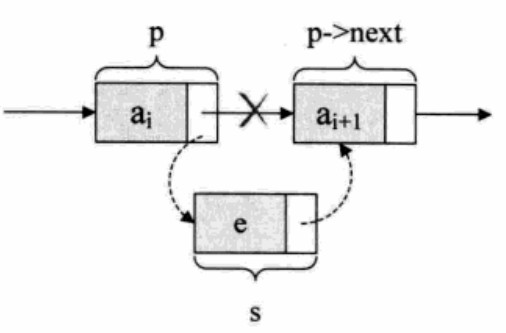
1. Insertion and deletion of single linked list:

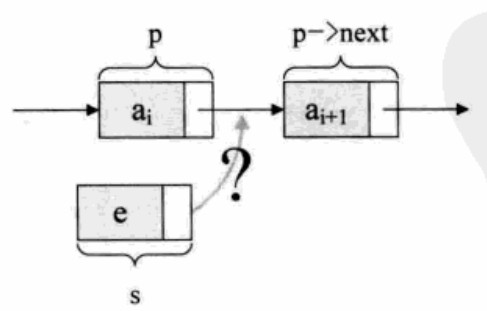
s->next = p->next;
p->next = s;

For the special case of the header and footer of a single linked list, the operation is the same:

//The ith data insertion node of the single linked list
Status ListInsert(LinkList *L,int i,ElemType e)
{
    LinkList p,s;
    p = *L; //Declare that a node p points to the first node in the linked list
    int j=1;
    //When p is not empty or j is not equal to i, the loop continues
    while (p && j<i)
    {
        p = p->next; //Assign the pointer field of the latter node to p
        ++j;
    }
    if (!p || j>i)
        return ERROR;
    s = (LinkList)malloc(sizeof(Node)); //Generate new node
    s->data = e;
    s->next = p->next;
    p-next = s;
}

1. Deletion of single linked list:

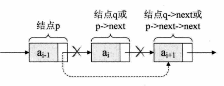
q = p->next;
p->next = q->next;

//Delete the ith data in the single linked list
Status ListDelete(LinkList *L,int i,ElemType *e)
{
    LinkList p,q;
    p = *L;
    int j=1;
    //As long as p - > next does not point to null and j < I, the loop continues
    while (p->next && j<i)
    {
        p = p->next;
        ++j;
    }
    //If P - > next points to null or j > I
    //Pay attention to understand why it is necessary to judge whether p - > next is empty, because p=*L is the header pointer, pointing to the header node rather than the first node
    if (!(p->next) || j>i)
        return ERROE; //The ith element does not exist
    q = p->next;
    p->next = q->next; //q is equivalent to a transition node
    *e = q->data;
    free(q); //Let the system reclaim the transition node to free memory
}

1. The whole table creation of a single linked table:

//Randomly generate the values of n elements and establish a single chain linear table L (head interpolation) of the leading node
void CreateListHead(LinkList *L,int n)
{
    LinkList p;
    int i;
    srand(time(0)); //Initialize random number seed
	*L = (LinkList)malloc(sizeof(Node));
    //Let the pointer of the head node of L point to NULL, that is, establish a single linked list of the head node
    (*L)->next = NULL; 
    for (i=0;i<n;i++)
    {
        p = (LinkList)malloc(sizeof(Node)); //Generate new node
        p->data = rand()%100+1; //Randomly generate numbers within 100
        p->next = (*L)->next;
        (*L)->next = p; //Insert into header
    }
}

//Randomly generate the values of n elements, and establish the single chain linear table L (tail interpolation) of the leading node
void CreateListTail(LinkList *L,int n)
{
    LinkList p,r;
    int i;
    srand(time(0));
    *L = (LinkList)malloc(sizeof(Node));
    r = *L; //r is the tail node, and r will change with the cycle
    for (i=0;i<n;i++)
    {
        p = (Node*)malloc(sizeof(Node)); //Generate new node
        p->data = rand()%100+1;
        r->next = p;
        r = p; //Loop change r to ensure that R is the tail node
    }
    //At the end of the loop, set the pointer field of the tail node of the linked list to null, so that the tail can be determined during subsequent traversal
    r->next = NULL; 
}

1. Delete the whole table of single linked list:

Status ClearList(LinkList *L)
{
    LinkList p,q;
    p = (*L)->next; //p points to the first node
    while (p) //It's not at the end of the watch
    {
        q = p->next;
        free(p);
        p = q;
    }
    (*L)->next = NULL; //Null header pointer field
}

1. Summary of single linked list structure and sequential storage structure:

(1) If the linear table needs frequent search and few insertion and deletion operations, the sequential storage structure should be adopted; If frequent insertion and deletion are required, the single linked list structure should be adopted.

(2) When the number of elements in the linear table changes greatly or the number of elements is not known at all, it is best to use the single linked list structure, because it does not need to consider the size of storage space; If the approximate length of the linear table is known in advance, the sequential storage structure is more efficient.

1. Static linked list:

(1) The linked list described by array is called static linked list

(2) Generally speaking, static linked list is actually a method to realize the ability of single linked list for high-level languages without pointers.

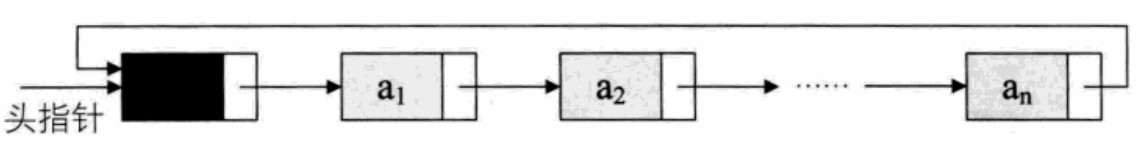
1. Circular linked list:

(1) Changing the pointer end of the terminal node in the single linked list from a null pointer to a head node makes the whole single linked list form a ring. This single linked list with head and tail connected is called a single cycle linked list, which is called a cycle linked list for short

(2) In order to make the processing of empty linked list consistent with that of non empty linked list, we usually set a header node. But it doesn't mean that a circular linked list must have a header node

(3) In a single linked list, if you have a head node, you can use O(1) time to access the first node, but for the access of the tail node, you need O(n) time; The tail pointer to the terminal node is used to represent the circular linked list, which is very convenient to find the first node and the terminal node

(4) Merge the two circular linked lists with the tail pointer rear:

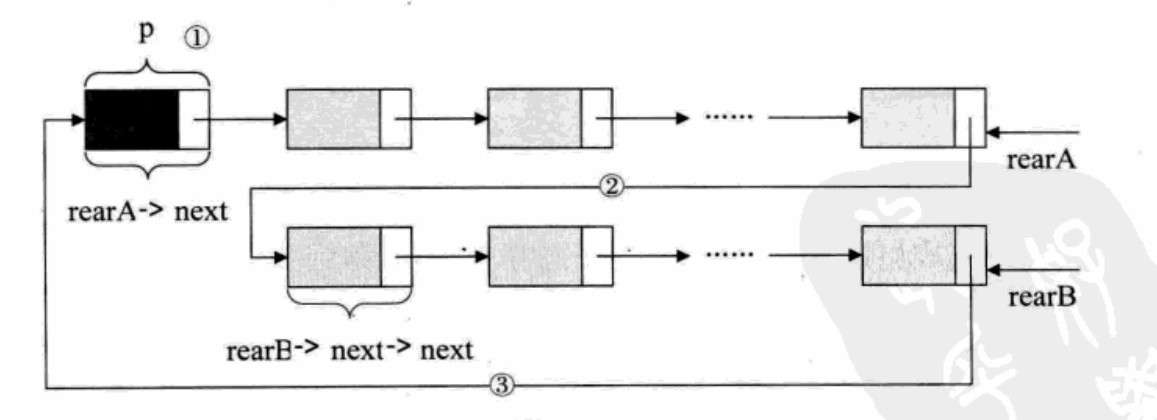
p = rearA->next; //Save the header node of table A
rearA->next = rearB->next->next; //Assign the first node (non header node) originally pointing to table B to Reala - > next
rearB->next = p; //Assign the header node of the original A table to realb - > next
free(p);

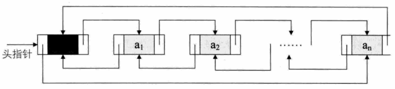
1. Bidirectional linked list:

(1) Bidirectional linked list is to set a pointer field to its predecessor node in each node of the single linked list

(2) Insertion of bidirectional linked list:

//Sequence is the key: first solve the precursor and successor of s, then the precursor of the later node, and finally solve the successor of the former node
s->prior = p;
s->next = p->next;
p->next->prior = s;
p->next = s;

(3) Deletion of bidirectional linked list:

p->prior->next = p->next;
p->next->prior = p->prior;
free(p);

(4) Summary:

A two-way linked list is more complex than a single linked list. It takes up more space because it needs to record two pointers. However, due to the good symmetry, it is more convenient to operate the front and back nodes of a node, and can effectively improve the time performance of the algorithm (exchanging space for time).

(to be continued...)