1. What is a data structure
1.1 some definitions of data structure
- "A data structure is a data object and the various relationships between the instances of the object and the data elements that make up the instance. These relationships can be given by defining relevant functions." Sartaj Sahni, data structure, algorithm and Application
- "Data structure is the physical implementation of ADT (Abstract Data Type)." Clifford A.Shaffer, data structure and algorithm analysis
- "Data Structure is a way of storing and organizing data in a computer. Usually, carefully selected data structures can lead to the most efficient algorithm." - Chinese Wikipedia
1.2 efficiency of problem solving methods
efficiency of problem solving methods: 1 It is related to the organization of data;
2. It is related to the utilization efficiency of space;
3. It has something to do with the cleverness of the algorithm.
1.2.1 it is related to the organization of data
example 1: how to place books on the bookshelf?
- Method 1: put it casually
Operation 1: how to insert a new book? Where there is time, put it in place in one step!
Operation 2: how to find a specified book? One by one, tired to death! - Method 2: search according to the alphabetical order of the book title
Operation 1: how to insert a new book? A new book "true story of Ah Q" starts with A. you need to move all the books behind it back
Operation 2: how to find a specified book? Binary search! - Method 3: divide the bookshelf into several areas. Each area is designated to place books of a certain category. In each category, they are placed according to the Pinyin alphabet of the book title
Operation 1: how to insert a new book? First determine the category, binary search, determine the position, and move out of the empty space
Operation 2: how to find a specified book? First determine the category, and then binary search
Question: how to allocate space? How detailed should the categories be?
example 1 tells us that the efficiency of problem-solving methods is related to the organization of data.
1.2.2 it is related to the utilization efficiency of space
example 2: write a program to implement a function PrintN, so that after passing in a parameter with a positive integer of N, all positive integers from 1 to n can be printed in sequence.
it is implemented by loop and recursion respectively, and the implementation code is as follows.
#include<iostream>
using namespace std;

//Loop implementation
void PrintN_Iteration(int n)
{
	for (int i = 1; i <= n; i++)
	{
		cout << i << endl;
	}
}

//Recursive implementation
void PrintN_Recursion(int n)
{
	if(n)
	{
		PrintN_Recursion(n - 1);
		cout << n << endl;
	}
}

int main()
{
	PrintN_Iteration(10000);
	//PrintN_Recursion(10000);

	system("pause");

	return 0;
}
test n=10, 100, 1000, 10000... Successively. When n=10000, the results of loop implementation and recursive implementation are shown in the figure below.
- Circular realization: it can print normally
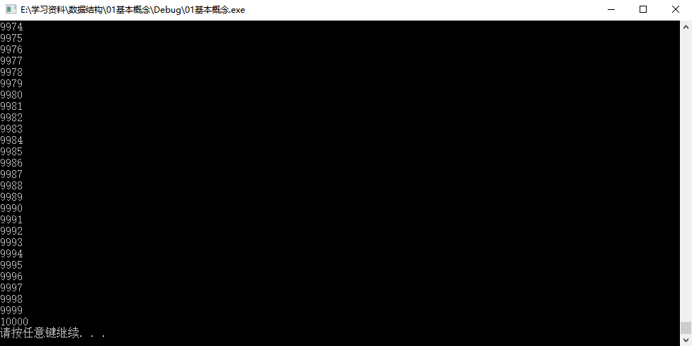
- Recursive implementation: there is an exception and it cannot print normally (it is not enough to use up all its available space, so there is an exception)

example 2 tells us that the efficiency of problem-solving methods is related to the efficiency of space utilization.
1.2.3 it is related to the cleverness of the algorithm
example 3: write a program to calculate a given polynomial f ( x ) = a 0 + a 1 x + . . . + a n − 1 x n − 1 + a n x n f(x)=a_{0}+a_{1}x+...+a_{n-1}x^{n-1}+a_{n}x^{n} f(x)=a0+a1x+...+ The value of an − 1 − xn − 1+an xn at a given point X.
the most direct method implementation code is as follows.
#include<iostream>
using namespace std;

double f1(double a[], int n, double x)
{
	double p = a[0];
	for (int i = 1; i <= n; i++)
	{
		p += (a[i] * pow(x, i));  //f(x)=a[0]+a[1]*x+...+a[n−1]*x^(n−1)+a[n]*x^(n)
	}
	return p;
}

int main()
{
	double a[] = { 0,1,2,3,4,5,6,7,8,9 };
	cout << "f1(1.1) = " << f1(9, a, 1.1) << endl;

	system("pause");

	return 0;
}
f1(1.1) = 84.0626
but generally, we will not use the above method to simplify f ( x ) = a 0 + a 1 x + . . . + a n − 1 x n − 1 + a n x n = a 0 + x ( a 1 + x ( . . . ( a n − 1 + x ( a n ) ) . . . ) ) f(x)=a_{0}+a_{1}x+...+a_{n-1}x^{n-1}+a_{n}x^{n}=a_{0}+x(a_{1}+x(...(a_{n-1}+x(a_{n}))...)) f(x)=a0+a1x+...+an−1xn−1+anxn=a0+x(a1+x(...(an−1+x(an))...)), Write the code as follows.
#include<iostream>
using namespace std;

double f2(double a[], int n, double x)
{
	double p = a[n];
	for (int i = n; i > 0; i--)
	{
		p = a[i - 1] + x * p;    //f(x)=a[0]+x*(a[1]+x*(...(a[n-1]+x*(a[n]))...))
	}
	return p;
}

int main()
{
	double a[] = { 0,1,2,3,4,5,6,7,8,9 };
	cout << "f2(1.1) = " << f2(9, a, 1.1) << endl;

	system("pause");

	return 0;
}
f2(1.1) = 84.0626
the second method is often used to calculate the given polynomial
f
(
x
)
=
a
0
+
a
1
x
+
.
.
.
+
a
n
−
1
x
n
−
1
+
a
n
x
n
f(x)=a_{0}+a_{1}x+...+a_{n-1}x^{n-1}+a_{n}x^{n}
f(x)=a0+a1x+...+ The value of an − 1 − xn − 1+an xn at a given point x is because the second method runs faster than the first method.
use the clock() timing function to record the program running time. The time unit is clock tick, that is, "time dot". The code for calculating the running time of the program written by the above two methods is as follows.
#include<iostream>
using namespace std;
#include<ctime>

double f1(double a[], int n, double x)
{
	double p = a[0];
	for (int i = 1; i <= n; i++)
	{
		p += (a[i] * pow(x, i));  //f(x)=a[0]+a[1]*x+...+a[n−1]*x^(n−1)+a[n]*x^(n)
	}
	return p;
}

double f2(double a[], int n, double x)
{
	double p = a[n];
	for (int i = n; i > 0; i--)
	{
		p = a[i - 1] + x * p;    //f(x)=a[0]+x*(a[1]+x*(...(a[n-1]+x*(a[n]))...))
	}
	return p;
}

int main()
{
	double a[] = { 0,1,2,3,4,5,6,7,8,9 };

	clock_t startTime, endTime;
	startTime = clock();//Timing start
	f1(a, 9, 1.1);
	endTime = clock();//End of timing
	cout << "The run time of f1 is: " << (double)(endTime - startTime) / CLOCKS_PER_SEC  << "s" << endl;  //Constant CLOCKS_PER_SEC counts the number of clocks that the machine clock goes per second
	cout << "f1(1.1) = " << f1(a, 9, 1.1) << endl;

	startTime = clock();//Timing start
    f2(a, 9, 1.1);
	endTime = clock();//End of timing
	cout << "The run time of f2 is: " << (double)(endTime - startTime) / CLOCKS_PER_SEC  << "s" << endl;
	cout << "f2(1.1) = " << f2(a, 9, 1.1) << endl;

	system("pause");

	return 0;
}
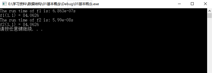
the running result of the code is shown in the figure below.

because the running speed is too fast, the results are all displayed as 0, so it is impossible to distinguish between speed and slow. Solution: let the measured function run repeatedly enough to make the measured total clock timing interval long enough. Finally, calculate the average running time of the measured function. Modify the code of the main function as follows.
int main()
{
	double a[] = { 0,1,2,3,4,5,6,7,8,9 };

	clock_t startTime, endTime;
	startTime = clock();//Timing start
	for (int i = 0; i < 1e7; i++)
	{
		f1(a, 9, 1.1);
	}
	//f1(a, 9, 1.1);
	endTime = clock();//End of timing
	//cout << "The run time of f1 is: " << (double)(endTime - startTime) / CLOCKS_PER_SEC  << "s" << endl;  // Constant CLOCKS_PER_SEC counts the number of clocks that the machine clock goes per second
	cout << "The run time of f1 is: " << (double)(endTime - startTime) / CLOCKS_PER_SEC / 1e7 << "s" << endl;
	cout << "f1(1.1) = " << f1(a, 9, 1.1) << endl;

	startTime = clock();//Timing start
	for (int i = 0; i < 1e7; i++)  //Call the function repeatedly to get enough clock beats
	{
		f2(a, 9, 1.1);
	}
	//f2(a, 9, 1.1);
	endTime = clock();//End of timing
	//cout << "The run time of f2 is: " << (double)(endTime - startTime) / CLOCKS_PER_SEC  << "s" << endl;
	cout << "The run time of f2 is: " << (double)(endTime - startTime) / CLOCKS_PER_SEC / 1e7 << "s" << endl;  //Calculate the single run time of the function
	cout << "f2(1.1) = " << f2(a, 9, 1.1) << endl;

	system("pause");

	return 0;
}
the running result of the code is shown in the figure below.
from the above results, it can be seen that the program written by the second method runs faster.
example 3 tells us that the efficiency of problem-solving methods is related to the cleverness of the algorithm.
1.3 what is a data structure
- Data structure is about the organization of data objects in the computer
⋄ \diamond ⋄ logical structure
⋄ \diamond ⋄ physical storage structure - The data object must be associated with a series of operations added to it
- The algorithm used to complete these operations
1.4 abstract data types
Abstract Data Type (ADT) is a mathematical model of a specific class of data structure with similar behavior in computer science; Or data types of one or more programming languages with similar semantics. Abstract Data Type is a theoretical tool to describe data structure. Its purpose is to enable people to understand the characteristics of data structure independent of the implementation details of the program. The definition of Abstract Data Type depends on its set of logical characteristics, and has nothing to do with how it is represented inside the computer.
- data type
⋄ \diamond ⋄ data object set
⋄ \diamond ⋄ operation set associated with the data set - Abstract: the method of describing data types does not depend on the concrete implementation
⋄ \diamond ⋄ independent of the machine where the data is stored
⋄ \diamond ⋄ independent of the physical structure of data storage
⋄ \diamond ⋄ it has nothing to do with the algorithm and programming language to realize the operation
it only describes the "what" of the data object set and related operation set, and does not involve the problem of "how to do it".
example 4: definition of abstract data type of "matrix".
∙
\bullet
∙ type name: matrix
∙
\bullet
∙ data object set: one
M
×
N
M\times N
M × Matrix of N
A
M
×
N
=
(
a
i
j
)
(
i
=
1
,
.
.
.
,
M
;
j
=
1
,
.
.
.
,
N
)
A_{M\times N}=(a_{ij})(i=1,...,M; j=1,...,N )
AM × N = (aij) (i=1,...,M;j=1,...,N)
M
×
N
M\times N
M × N triples
<
a
,
i
,
j
>
<a, i, j >
< A, I, J > composition, where
a
a
a is the value of the matrix element,
i
i
i is the line number of the element,
j
j
j is the column number of the element.
∙
\bullet
· operation set: for any matrix
A
A
A,
B
B
B,
C
C
C
∈
\in
∈ Matrix, and integer
i
i
i,
j
j
j,
M
M
M,
N
N
N
∘
\circ
∘ matrix create (int m, int n): returns a
M
×
N
M\times N
M × Empty matrix of N;
∘
\circ
∘ int getmaxrow (matrix A): returns the total number of rows of matrix A;
∘
\circ
∘ int getmaxcol (matrix A): returns the total number of columns of matrix A;
∘
\circ
∘ ElementType GetEntry (Matrix A, int i, int j): returns the elements in row I and column J of matrix A;
∘
\circ
∘ Matrix Add (Matrix A, Matrix B): if the number of rows and columns of a and B are the same, the matrix C=A+B is returned; otherwise, the error flag is returned;
∘
\circ
∘ Matrix Multiply (Matrix A, Matrix B): if the number of columns of a is equal to the number of rows of B, the matrix C=AB is returned; otherwise, the error flag is returned;
∘
\circ
∘ ... ...
abstract representation: 1 In the data object set, a is only the value of the matrix element and does not care about its specific data type;
2. In the operation set, ElementType GetEntry (Matrix A, int i, int j) also returns a general data type ElementType, not a specific data type.
2. What is an algorithm
2.1 definitions
∙
\bullet
∙ Algorithm
∘
\circ
∘ a finite instruction set
∘
\circ
∘ accept some input (in some cases, no input is required)
∘
\circ
∘ generate output
∘
\circ
∘ must terminate after limited steps
∘
\circ
∘ each instruction must
⋄
\diamond
⋄ have fully clear objectives, and there can be no ambiguity
⋄
\diamond
⋄ within the range that the computer can handle
⋄
\diamond
⋄ the description should not depend on any computer language and specific implementation means
example 1: select the pseudo code description of the sorting algorithm.
//List N integers [0] List [N-1] for non decreasing sort
void SelectionSort(int List[], int N)
{
    for(int i = 0; i < N; i++)
    {
        MinPosition = ScanForMin(List, i ,N-1);  //Find the smallest element from List[i] to List[N-1] and assign its position to MinPosition

        Swap(List[i], List[MinPosition]);  //Change the smallest element of the unordered part to the last position of the ordered part
    }
}
a very important feature of the above pseudo code description is abstraction, which is reflected in the following points:
- Is List an array or a linked List?
- Is Swap implemented with functions or macros?
the above two points are the details of specific implementation, which are not concerned when describing the algorithm.
2.2 indicators to measure the quality of the algorithm
what is a good algorithm? Generally, the following two indicators can be used to measure:
- Space complexity S(n): the length of the storage unit occupied by the program written according to the algorithm during execution. This length is often related to the size of the input data. Algorithms with too high space complexity may cause the memory used to exceed the limit, resulting in abnormal program interruption.
- The length of time spent in the execution of the program (T): according to the complexity of the algorithm. This length is often related to the size of the input data. Inefficient algorithms with high time complexity may cause us to wait for running results in our lifetime.
2.2.1 space complexity S(n)
example 2: for the recursive implementation of the previously written PrintN function, there will be an exception when n=10000, and the reason why it cannot print normally is analyzed.
//Recursive implementation
void PrintN_Recursion(int n)
{
	if(n)
	{
		PrintN_Recursion(n - 1);
		cout << n << endl;
	}
}
for the above recursive implementation code, if you want to run PrintN(100000), before calling PrintN(99999), you need to store all the states of the PrintN(100000) function in the system memory, then execute PrintN(99999), call and execute successively until the call PrintN(0) returns, as shown in the following figure.
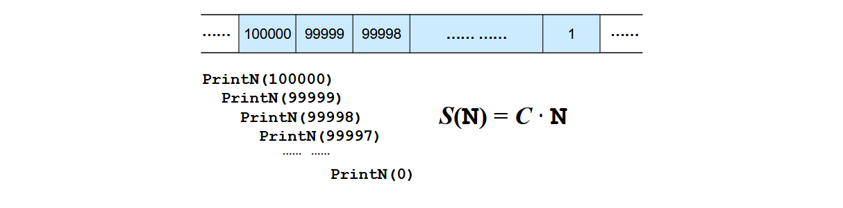
spatial complexity
S
(
N
)
=
C
⋅
N
S(N) = C \cdot N
S(N)=C ⋅ N and length
N
N
N is proportional when
N
N
When N is very large, the space that the program can use is limited, so the program will explode.
//Loop implementation
void PrintN_Iteration(int n)
{
	for (int i = 1; i <= n; i++)
	{
		cout << i << endl;
	}
}
for the above loop implementation, there is no call, so no matter N N How big N is, the memory occupied is always a fixed value, which will not change with the time N N N increases, so the program will run normally.
2.2.2 time complexity T(n)
example 3: for the program previously written to calculate the value of polynomial at a given point x, the reason why the first method is slower than the second method is analyzed.
when analyzing the operation efficiency of a function, if there is only addition, subtraction, multiplication and division, the machine runs the addition and subtraction method much faster than the multiplication and division method, so it is basically calculating the times of all multiplication and division methods of the function, and the addition and subtraction method can be ignored.
double f1(double a[], int n, double x)
{
	double p = a[0];
	for (int i = 1; i <= n; i++)
	{
		p += (a[i] * pow(x, i));  //f(x)=a[0]+a[1]*x+...+a[n−1]*x^(n−1)+a[n]*x^(n)
	}
	return p;
}
for the implementation code of the first method above, each time the for loop is executed, a[i] * pow(x, i) performs one multiplication, pow(x, i) performs i-1 multiplication, a total of I multiplication is executed, and the for loop is executed n times, so it is executed in total 1 + 2 + . . . + n = n 2 + n 2 1+2+...+n=\frac{n^{2}+n}{2} 1+2+...+n=2n2+n times multiplication, time complexity is T ( n ) = C 1 n 2 + C 2 n T(n)=C_{1}n^{2}+C_{2}n T(n)=C1n2+C2n.
double f2(double a[], int n, double x)
{
	double p = a[n];
	for (int i = n; i > 0; i--)
	{
		p = a[i - 1] + x * p;    //f(x)=a[0]+x*(a[1]+x*(...(a[n-1]+x*(a[n]))...))
	}
	return p;
}
for the implementation code of the second method above, each time the for loop is executed, p = a[i - 1] + x * p performs multiplication once, and the for loop is executed n times in total, so it is executed in total n n n times of multiplication, the time complexity is T ( n ) = C ⋅ n T(n)=C \cdot n T(n)=C⋅n.
when n is large enough, T ( n ) = C 1 n 2 + C 2 n T(n)=C_{1}n^{2}+C_{2}n The time complexity of T(n)=C1 , n2+C2 , n is much greater than T ( n ) = C ⋅ n T(n)=C \cdot n T(n)=C⋅n.
when analyzing the efficiency of general algorithms, we often pay attention to the following two complexities:
- Worst case complexity T ( w o r s t ) ( n ) T_{(worst)}(n) T(worst)(n)
- Average complexity T ( a v g ) ( n ) T_{(avg)}(n) T(avg)(n)
T ( a v g ) ( n ) < T ( w o r s t ) ( n ) T_{(avg)}(n)<T_{(worst)}(n) T(avg) (n) < T (worst) (n). Generally, more attention is paid to the complexity of the worst case.
2.3 progressive representation of complexity
when we analyze the complexity of the algorithm, we only care about the nature that the complexity increases with the increase of the scale of the data to be processed. There is no need for fine analysis, so we need a progressive representation of the complexity.
∙
\bullet
∙
T
(
n
)
=
O
(
f
(
n
)
)
T(n)=O(f(n))
T(n)=O(f(n)) indicates the existence of a constant
C
>
0
C>0
C>0,
n
0
>
0
n_{0} >0
n0 > 0, properly
n
≥
n
0
n ≥ n_{0}
When n ≥ n0 , yes
T
(
n
)
≤
C
⋅
f
(
n
)
T ( n ) ≤ C ⋅ f ( n )
T(n) ≤ C ⋅ f(n), i.e
O
(
f
(
n
)
)
O(f(n))
O(f(n)) indicates
f
(
n
)
f(n)
f(n) yes
T
(
n
)
T(n)
Some upper bound of T(n);
∙
\bullet
∙
T
(
n
)
=
Ω
(
g
(
n
)
)
T(n)=Ω(g(n))
T(n) = Ω (g(n)) indicates the existence of a constant
C
>
0
C>0
C>0,
n
0
>
0
n_{0} >0
n0 > 0, properly
n
≥
n
0
n ≥ n_{0}
When n ≥ n0 , yes
T
(
n
)
≤
C
⋅
g
(
n
)
T ( n ) ≤ C ⋅ g ( n )
T(n) ≤ C ⋅ g(n), i.e
Ω
(
g
(
n
)
)
Ω(g(n))
Ω (g(n)) indicates
g
(
n
)
g(n)
g(n) yes
T
(
n
)
T(n)
Some lower bound of T(n);
∙
\bullet
∙
T
(
n
)
=
Θ
(
h
(
n
)
)
T(n) = \Theta(h(n))
T(n)= Θ (h(n)) indicates simultaneous
T
(
n
)
=
O
(
h
(
n
)
)
T ( n ) = O ( h ( n ) )
T(n)=O(h(n)) and
T
(
n
)
=
Ω
(
h
(
n
)
)
T(n) = Ω(h(n))
T(n) = Ω (h(n)), i.e
Θ
(
h
(
n
)
)
\Theta(h(n))
Θ (h(n)) indicates
h
(
n
)
h(n)
h(n)
T
(
n
)
T(n)
The upper bound of T(n) is also the lower bound.
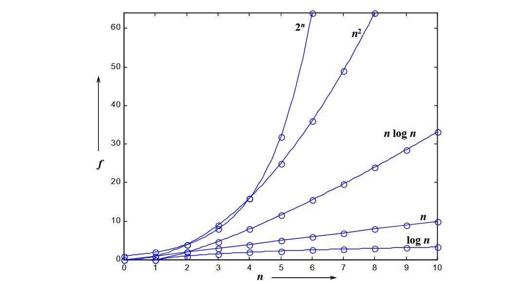
the following table shows the growth rate of complexity of different functions with the growth of n n ! n! n! The complexity of is growing fastest.
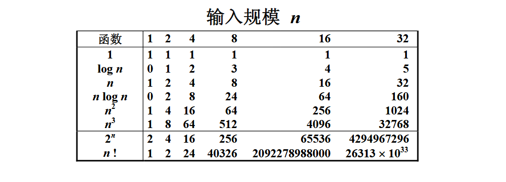
the following figure shows the growth rate of complexity of different functions with the growth of n
l
o
g
n
logn
logn is the best function.
2.4 complexity analysis tips
∙
\bullet
∙ if the two algorithms have complexity respectively
T
1
(
n
)
=
O
(
f
1
(
n
)
)
T_{1} ( n ) = O ( f_{1} ( n ) )
T1 (n)=O(f1 (n)) and
T
2
(
n
)
=
O
(
f
2
(
n
)
)
T_{2} ( n ) = O ( f_{2} ( n ) )
T2 (n)=O(f2 (n)), then
∘
\circ
∘
T
1
(
n
)
+
T
2
(
n
)
=
m
a
x
(
O
(
f
1
(
n
)
)
,
O
(
f
2
(
n
)
)
)
T_{1}( n ) + T_{2}( n ) = max ( O ( f_{1} ( n ) ), O ( f_{2} ( n ) ) )
T1(n)+T2(n)=max(O(f1(n)),O(f2(n)))
∘
\circ
∘
T
1
(
n
)
×
T
2
(
n
)
=
O
(
f
1
(
n
)
×
f
2
(
n
)
)
T_{1} ( n ) ×T_{2} ( n ) = O (f_{1}( n ) ×f_{2} ( n ) )
T1(n)×T2(n)=O(f1(n)×f2(n))
∙
\bullet
∙ if
T
(
n
)
T(n)
T(n) is about
n
n
n
k
k
k-order polynomial, then
T
(
n
)
=
Θ
(
n
k
)
T ( n ) = \Theta ( n^{k} )
T(n)=Θ(nk).
∙
\bullet
· the time complexity of a for loop is equal to the number of loops multiplied by the complexity of the loop body code.
∙
\bullet
· the complexity of the if else structure depends on the conditional judgment complexity of the if and the complexity of the two branches, and the overall complexity is the largest of the three
3. Application examples: maximum child columns and problems
sequence of given N integers { A 1 , A 2 , . . . , A N } \{ A_{1}, A_{2}, ..., A_{N} \} {A1, A2,..., AN}, find the function f ( i , j ) = m a x { 0 , ∑ k = i j A k } f(i,j)=max\{0, \sum ^{j}_{k=i}A_{k} \} f(i,j)=max{0, ∑ k=ij, Ak}.
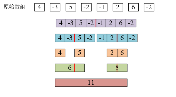
analysis: "continuous sub column" is defined as { N i , N i + 1 , ... , N j } \{ N_{i} , N_{i+1} , ..., N_j \} {N I, N i+1,..., Nj}, where 1 ≤ I ≤ j ≤ K. "Maximum child column sum" is defined as the largest sum of all continuous child column elements. For example, for a given sequence {4, - 3, 5, - 2, - 1, 2, 6, - 2}, its continuous child columns {4, - 3, 5, - 2, - 1, 2, 6} have the largest sum and 11.
- Algorithm 1: determine the head and tail of the sub column, and then traverse and accumulate. The time complexity is O ( n 3 ) O(n^3) O(n3)
//Algorithm 1: determine the head and tail of the sub column, and then traverse and accumulate. The time complexity is O(n^3)
#include<iostream>
using namespace std;

int MaxSubseqSum1(int a[], int n)
{
	int ThisSum, MaxSum = 0;
	for (int i = 0; i < n; i++)  //i is the position of the left end of the sub column
	{
		for (int j = 0; j < n; j++)  //j is the right end of the sub column
		{
			ThisSum = 0;  //ThisSum is the sum of the child columns from a[i] to a[j]
			for (int k = i; k <= j; k++)
			{
				ThisSum += a[k];
			}
			if (ThisSum > MaxSum)  //If the sum of the newly obtained sub column is larger, the result will be updated
			{
				MaxSum = ThisSum;
			}
		}
	}
	return MaxSum;
}

int main() {
	int n;
	int a[100000 + 5];
	cout << "Please enter the length of the child column n: " << endl;
	cin >> n;  // 8
	cout << "Please enter the elements of the child column (separated by spaces):" << endl;
for (int i = 0; i < n; i++)
	{
		cin >> a[i];  // a[]={ 4, -3, 5, -2, -1, 2, 6, -2 };
	}
	cout << "Maximum child column sum:" << endl;
	int MaxSum1 = MaxSubseqSum1(a, n);  // 11
	cout << "Algorithm 1 Result:" << MaxSum1 << endl;

	system("pause");

	return 0;
}
Please enter the length of the sub column n:
8
Please enter the elements of the child column (separated by spaces):
4 -3 5 -2 -1 2 6 -2
Maximum child column sum:
Algorithm 1 Result: 11
- Algorithm 2: determine the head of the sub column, accumulate one by one, and the time complexity is O ( n 2 ) O(n^2) O(n2)
//Algorithm 2: determine the header of the sub columns, accumulate them one by one, and the time complexity is O(n^2)
#include<iostream>
using namespace std;

int MaxSubseqSum1(int a[], int n)
{
	int ThisSum, MaxSum = 0;
	for (int i = 0; i < n; i++)  //i is the position of the left end of the sub column
	{
		ThisSum = 0;  //ThisSum is the sum of the child columns from a[i] to a[j]
		for (int j = i; j < n; j++)  //j is the right end of the sub column
		{
			ThisSum += a[j];
			if (ThisSum > MaxSum)  //If the sum of the newly obtained sub column is larger, the result will be updated
			{
				MaxSum = ThisSum;
			}
		}
	}
	return MaxSum;
}

int main() {
	int n;
	int a[100000 + 5];
	cout << "Please enter the length of the child column n: " << endl;
	cin >> n;  // 8
	cout << "Please enter the elements of the child column (separated by spaces):" << endl;
	for (int i = 0; i < n; i++)
	{
		cin >> a[i];  // a[]={ 4, -3, 5, -2, -1, 2, 6, -2 };
	}
	cout << "Maximum child column sum:" << endl;
	int MaxSum2 = MaxSubseqSum2(a, n);  // 11
	cout << "Algorithm 2 Result:" << MaxSum2 << endl;

	system("pause");

	return 0;
}
Please enter the length of the sub column n:
8
Please enter the elements of the child column (separated by spaces):
4 -3 5 -2 -1 2 6 -2
Maximum child column sum:
Algorithm 2 Result: 11
- Algorithm 3: divide and conquer. In short, it is to decompose a large problem into several small problems, and then find the optimal solution from the solutions of all small problems. For this problem, a large sequence can be divided into two small sequences, and then the small sequence can be divided into two smaller sequences,... Until each small sequence has only one number, which is the process of division. In each small sequence, you will get:
1. The sum of the largest child columns on the left (positive number is itself, negative number is 0);
2. The sum of the largest child columns on the right;
3. The sum of the largest child columns across the partition boundary.
At this time, the largest value of the three is the "maximum sub column sum" of the small sequence, so as to obtain the "maximum sub column sum" of the larger sequence, and finally obtain the maximum sub column sum of the whole sequence.
The time complexity is T ( n ) = 2 T ( n 2 ) + c ⋅ n , T ( 1 ) = O ( 1 ) = 2 [ 2 T ( n 2 2 ) + c ⋅ n 2 ] + c ⋅ n = 2 k O ( 1 ) + + c ⋅ k ⋅ n , his in n 2 k = 1 ⇒ k = l o g n = O ( n l o g n ) \begin{matrix} T ( n ) = 2 T (\frac{n}{2}) + c ⋅ n , & T ( 1 ) = O ( 1 ) \ _ {}\ _ {}\ _ {}\ _ {}\ _ {}\ _ {}\ _ {}\ _ {}\ _ {}\ _ {}\ _ {}\ _ {}\ _ {}\ _ {}\ _ {}\ \ _ {}\ _ {}\ _ {}\ _ {}\ _ {}\ _ {}\ _ {}\ _ {}\ _ {}\ _ {}\ _ {}\ _ {}\ _ {}\ _ {}\ _ {}\ _ {}\ _ {}\ _ {}\ _ {}\ _ {}\ _ {}=2[2T(\frac{n}{2^{2}})+ c ⋅\frac{ n}{2}] +c ⋅n& \ \ _ {}\ _ {}\ _ {}\ _ {}\ _ {}\ _ {}\ _ {}\ _ {}\ _ {}\ _ {}\ _ {}\ _ {}\ _ {}\ _ {}\ _ {}\ _ {}\ _ {}\ _ {}\ _ {}= 2^{k}O(1) ++ c ⋅ k⋅n,\ _ {}\ _ {}\ _ {} & where \ frac {n} {2 ^ {K}} = 1 \ rightarrow k = logn \ \ \_ {}\ _ {}=O(nlogn) \end{matrix} T(n)=2T(2n)+c⋅n, =2[2T(22n)+c⋅2n]+c⋅n =2kO(1)++c⋅k⋅n, ⇒ where t (NLO) = 2kn (NLO) = 1
//Algorithm 3: divide and conquer, recursively divide into two parts, calculate the maximum sum of sub columns after each segmentation, and the time complexity is O(nlogn)
//Returns the maximum of the left largest child column sum, the right largest child column sum, the largest child column across the partition boundary, and the maximum of the three
int MaxSum(int A, int B, int C)
{
	return (A > B) ? ((A > C) ? A : C) : ((B > C) ? B : C);
}
//Divide and conquer
int DivideAndConquer(int a[], int left, int right)
{
	if (left == right) 	//Recursion end condition: the child column has only one number
	{
		if (a[left] > 0)  // When the number is positive, the maximum child column sum is itself
		{
			return a[left];
		}
		return 0;	// When the number is negative, the maximum child column sum is 0
	}

	//Recursively find the left and right largest sub columns and
	int mid = left + (right - left) / 2;  //Using left+(right - left)/2 to calculate mid is to prevent integer overflow
	int MaxLeftSum = DivideAndConquer(a, left, mid);
	int MaxRightSum = DivideAndConquer(a, mid + 1, right);

	//Then find the sum of the left and right cross-border largest sub columns respectively
	int MaxLeftBorderSum = 0;
	int LeftBorderSum = 0;
	for (int i = mid; i >= left; i--)  //We should start from the border and look to the left
	{
		LeftBorderSum += a[i];
		if (LeftBorderSum > MaxLeftBorderSum)
			MaxLeftBorderSum = LeftBorderSum;
	}
	int MaXRightBorderSum = 0;
	int RightBorderSum = 0;
	for (int i = mid + 1; i <= right; i++)  // Start from the border and look to the right
	{
		RightBorderSum += a[i];
		if (RightBorderSum > MaXRightBorderSum)
			MaXRightBorderSum = RightBorderSum;
	}

	//Finally, it returns the sum of the left largest sub column, the right largest sub column, and the cross-border largest sub column and the largest number of the three
	return MaxSum(MaxLeftSum, MaxRightSum, MaXRightBorderSum + MaxLeftBorderSum);
}
int MaxSubseqSum3(int a[], int n)
{
	return DivideAndConquer(a, 0, n - 1);
}

int main() {
	int n;
	int a[100000 + 5];
	cout << "Please enter the length of the child column n: " << endl;
	cin >> n;  // 8
	cout << "Please enter the elements of the child column (separated by spaces):" << endl;
for (int i = 0; i < n; i++)
	{
		cin >> a[i];  // a[]={ 4, -3, 5, -2, -1, 2, 6, -2 };
	}
	cout << "Maximum child column sum:" << endl;
	int MaxSum3 = MaxSubseqSum3(a, n);  // 11
	cout << "Algorithm 3 Result:" << MaxSum3 << endl;

	system("pause");

	return 0;
}
Please enter the length of the sub column n:
8
Please enter the elements of the child column (separated by spaces):
4 -3 5 -2 -1 2 6 -2
Maximum child column sum:
Algorithm 3 Result: 11
- Algorithm 4: online processing. "Online" means that every time a data is input, it will be processed immediately. If the input is stopped anywhere, the algorithm can correctly give the current solution. The time complexity is O ( n ) O(n) O(n).
//Algorithm 4: online processing, direct accumulation. If the sum accumulated to the current is negative, set the current value or 0, and the time complexity is O(n)
int MaxSubseqSum4(int a[], int n)
{
	int ThisSum = 0;
	int MaxSum = 0;
	for (int i = 0; i < n; i++)
	{
		ThisSum += a[i];
		if (ThisSum < 0)
		{
			ThisSum = 0;
		}
		else if (ThisSum > MaxSum)
		{
			MaxSum = ThisSum;
		}
	}
	return MaxSum;
}

int main() {
	int n;
	int a[100000 + 5];
	cout << "Please enter the length of the child column n: " << endl;
	cin >> n;  // 8
	cout << "Please enter the elements of the child column (separated by spaces):" << endl;
for (int i = 0; i < n; i++)
	{
		cin >> a[i];  // a[]={ 4, -3, 5, -2, -1, 2, 6, -2 };
	}
	cout << "Maximum child column sum:" << endl;
	int MaxSum4 = MaxSubseqSum4(a, n);  // 11
	cout << "Algorithm 4 Result:" << MaxSum4 << endl;

	system("pause");

	return 0;
}
Please enter the length of the sub column n:
8
Please enter the elements of the child column (separated by spaces):
4 -3 5 -2 -1 2 6 -2
Maximum child column sum:
Algorithm 4 Result: 11
on a certain machine, the running time comparison results of the four algorithms under different input scales are shown in the figure below.

it can be seen that the fourth algorithm is the best. When n = 100000, the operation result can still be obtained in less than 1 second.