Data structure:
  data structure is the way that computers store and organize data. It refers to the collection of data elements with one or more specific relationships
Algorithm:
  algorithm is a well-defined calculation process. It takes one or a group of values as input and generates one or a group of values as output The so-called programming is data structure (storage form of data) plus algorithm (packaging of a series of steps)

Time complexity

  definition of time complexity: in computer science, the time complexity of an algorithm is a function that quantitatively describes the running time of the algorithm. In theory, the time spent in the execution of an algorithm cannot be calculated. You can only know when you put your program on the machine and run it. But do we need every algorithm to be tested on the computer? Yes, it can be tested on the computer, but it is very troublesome, so there is the analysis method of time complexity. The time spent by an algorithm is directly proportional to the execution times of the statements in it. The execution times of the basic operations in the algorithm is the time complexity of the algorithm.

To put it simply: time complexity is the number of times a basic operation is executed

Time complexity instance

Example:

The code is as follows (example):

Please calculate how many times the Func1 basic operation is executed?

void Func1(int N)
{
	int count = 0;
	for (int i = 0; i < N ; ++ i){
		for (int j = 0; j < N ; ++ j){
			++count;
		}
	}
	for (int k = 0; k < 2 * N ; ++ k){
		++count;
	}
	int M = 10;
	while (M--){
	++count;
	}
	printf("%d\n", count);
}

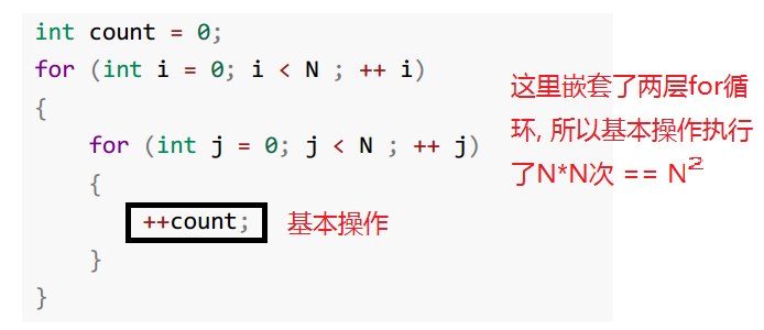
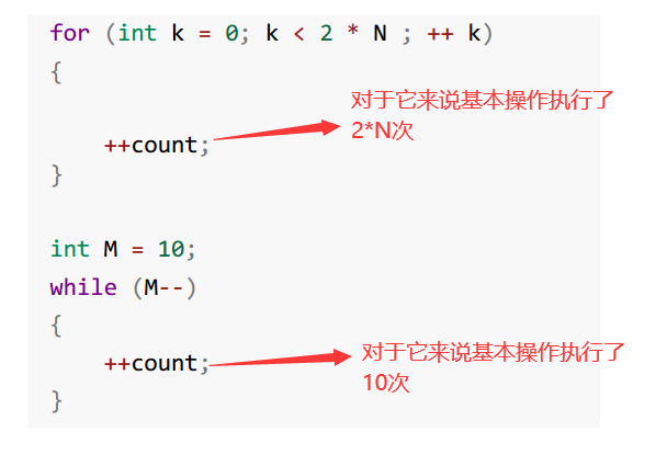
In this code, adding "+ + count" is a basic operation, which is an instruction

So for this code, its time complexity is N^2;

Number of basic operations performed by Func1:
F(N) = N^2 + 2*N + 10

• N = 10 F(N) = 130
• N = 100 F(N) = 10210
• N = 1000 F(N) = 1002010

In fact, when we calculate the time complexity, we do not have to calculate the exact execution times, but only the approximate execution times. Here, we use the asymptotic representation of large O.
Derivation of large O-order method:
1. Replace all addition constants in the run time with constant 1. (the asymptotic time complexity of any constant term is an O(1) time complexity)

2. In the modified run times function, only the highest order term is retained. (the highest order term will directly affect the time of our algorithm. If there are coefficients in front of the highest order term, the coefficients can also be removed)

3. If the highest order term exists and is not 1, the constant multiplied by this item is removed. The result is large O-order.
After using the asymptotic representation of large o, the time complexity of Func1 is O(N^2)

• N = 10 F(N) = 100
• N = 100 F(N) = 10000
• N = 1000 F(N) = 1000000

From the above, we can find that the progressive representation of big O removes those items that have little impact on the results, and succinctly represents the execution times.
Evaluate the quality of an algorithm and adopt the worst time complexity;

practice:

void Func2(int N)
{
	int count = 0;
	for (int k = 0; k < 2 * N ; ++ k){
		++count;
	}
	int M = 10;
	while (M--){
		++count;
	}
	printf("%d\n", count);
}

void Func3(int N, int M)
{
	int count = 0;
	for (int k = 0; k < M; ++ k){
		++count;
	}
	for (int k = 0; k < N ; ++ k){
		++count;
	}
	printf("%d\n", count);
}

void Func4(int N)
{
	int count = 0;
	for (int k = 0; k < 100; ++ k){
		++count;
	}
	printf("%d\n", count);
}

const char * strchr ( const char * str, int character );

void BubbleSort(int* a, int n)
{
	assert(a);
	for (size_t end = n; end > 0; --end){
		int exchange = 0;
		for (size_t i = 1; i < end; ++i){
			if (a[i-1] > a[i]){
				Swap(&a[i-1], &a[i]);
				exchange = 1;
			}
		}
		if (exchange == 0)
		break;
	} 
}

int BinarySearch(int* a, int n, int x)
{
	assert(a);
	int begin = 0;
	int end = n-1;
	while (begin < end){
		int mid = begin + ((end-begin)>>1);
		if (a[mid] < x)
			begin = mid+1;
		else if (a[mid] > x)
			end = mid;
		else
		return mid;
	}
	return -1;
}

long long Factorial(size_t N)
{
	return N < 2 ? N : Factorial(N-1)*N;
}

long long Fibonacci(size_t N)
{
return N < 2 ? N : Fibonacci(N-1)+Fibonacci(N-2);
}

Example answer and analysis:

1. The basic operation of example 1 was performed 2N+10 times. It is known that the time complexity is O(N) by deriving the large O-order method
2. The basic operation of example 2 is executed M+N times, with two unknowns M and N, and the time complexity is O(N+M)
3. The basic operation of example 3 is performed 10 times. By deriving the large O-order method, the time complexity is O(1)
4. In example 4, the basic operation is executed for the best time and the worst N times. The time complexity is generally the worst, and the time complexity is O(N)
5. In example 5, the basic operation is executed for the best N times and the worst (N*(N+1)/2 times. By deriving the large O-order method + time complexity, it is generally the most important
   Bad, time complexity is O(N^2)
6. In example 6, the basic operation is performed for the best time and the worst time. The time complexity is O(logN) ps: logN is the bottom in algorithm analysis
   The number is 2 and the logarithm is N. Some places will be written as lgN. (it is suggested to explain how logN is calculated through origami search)
7. In Example 7, through calculation and analysis, it is found that the basic operation recurses N times and the time complexity is O(N).
8. Example 8 shows that the basic operation recurses 2^N times and the time complexity is O(2^N). (it is recommended to draw a binary tree of recursive stack frames
   Explanation)

Time complexity

Space complexity is a measure of the amount of storage space temporarily occupied by an algorithm during operation. Space complexity is not how many bytes the program occupies, because it doesn't make much sense, so space complexity is the number of variables. The calculation rules of spatial complexity are basically similar to the practical complexity, and the large O asymptotic representation is also used.

The number of variables determines its spatial complexity

Example:

void BubbleSort(int* a, int n)
{
	assert(a);
	for (size_t end = n; end > 0; --end)
	{
		int exchange = 0;
		for (size_t i = 1; i < end; ++i)
		{
			if (a[i-1] > a[i])
			{
				Swap(&a[i-1], &a[i]);
				exchange = 1;
			}
		}
		if (exchange == 0)
		break;
	}
}

long long* Fibonacci(size_t n)
{
	if(n==0)
		return NULL;
	long long * fibArray =(long long *)malloc((n+1) * sizeof(long long));
	fibArray[0] = 0;
	fibArray[1] = 1;
	for (int i = 2; i <= n ; ++i)
	{
		fibArray[i ] = fibArray[ i - 1] + fibArray [i - 2];
	}
	return fibArray ;
}

long long Factorial(size_t N)
{
	return N < 2 ? N : Factorial(N-1)*N;
}

Example answer and analysis:

1. Example 1 uses an additional space, so the space complexity is O(1)
2. Example 2 dynamically opens up N spaces, and the space complexity is O(N)
3. Example 3 recursively called N times, opened up N stack frames, and each stack frame used a constant space. Space complexity is O(N)