Linear table
Definition and characteristics of linear table
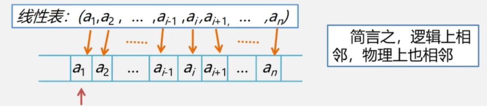
A linear table is a finite sequence of data elements with the same characteristics.
Linear list: an ordered sequence composed of n (n > = 0) data elements (nodes) a1,a1,... An.
definition:
1. The number n of data elements is defined as the length of the table.
2. When n=0, it is called an empty table.
3. Record the non empty linear table (n > 0) as: (a1,a2,... an)
4. The data element AI (I < = I < = n) here is just an abstract symbol, and its specific meaning can be different in different cases.
Logical characteristics of linear table
1. In a non empty linear table, there is and only one start node a1, which has no direct precursor but only one direct successor a2;
2. There is only one terminal node an, which has no direct successor, but only one direct precursor an-1;
3. The other internal nodes AI (2 < = I < = n-1) have only one direct precursor ai-1 and one direct successor a+1.
Sequence table
The sequential representation of linear table is also called sequential storage structure or sequential image.
Definition of sequence table
A storage structure that stores logically adjacent data elements in physically adjacent storage units.
Number address
Each storage unit in the memory has its own number, which is called the address.
Calculation of storage location
Assuming that each element of the linear table needs to occupy L storage units, the relationship between the storage location of the i+1 data element and the storage location of the i data element satisfies:
LOC(ai+1) = LOC(ai) + L
Thus, the storage locations of all data elements can be obtained from the storage location of the first data element:
LOC(ai) = LOC(a1) + (i-1) * L
Access operation time performance
Through this formula, the address of any position in the linear table can be calculated at any time. Whether it is the first or the last, it is the same time, that is, for the storage or extraction of data at each position of the linear table, it is the same time for the computer, that is, a constant time. Therefore, the access operation time performance of the linear table is O(1).
Random storage structure
We usually call the storage structure with constant performance O(1) of access operation as random storage structure.
Time complexity
(1) For access operations
The sequential storage structure of linear table. For access operation, its time complexity is O(1)
Because the element position can be calculated directly.
(2) For insert and delete operations
For insert and delete operations, the time complexity is O(n)
Because after insertion or deletion, the remaining elements need to be moved.
Usage scenario
The linear table sequential storage structure is more suitable for scenarios with more element access operations and less addition and deletion operations.
Creation of sequence table
#define MAXSIZE 100
typedef struct{
    ElemType elem[MAXSIZE];
    int length;
}SqList;    //static state
typedef struct{
    ElemType *elem;
    int length;
}SqList;
L.elem = (ElemType*)malloc(size(ElemType)*MAXSIZE);   //dynamic
Main algorithm
Algorithm 1: initialization of linear table L
Status InitList_Sq(SqList &L){			//Construct an empty sequence table L
    L.elem = new ElemType[MAXSIZE];		//Allocate space for sequential tables
    if(!L.elem)							//Storage allocation failed
        exit(OVERFLOW);
    L.length = 0;						//Empty table length is 0
    return Ok;
}
Algorithm 2: destroy linear table L
void DestroyList(SqList &L){
	if(L.elem)
		delete L.elem;	//Free up storage space
}
Algorithm 3: empty linear table L
void ClearList(SqList &L){
    L.length = 0;
}
Algorithm 4: find the length of linear table L
int GetLength(SqList L){
    return(L.length);
}
Algorithm 5: judge whether the linear table L is empty
int IsEmpty(SqList L){
	if(L.length == 0)
        return 1;
    return 0;
}
Algorithm 6: value of sequence table (obtain the content of corresponding location data element according to location i)
int GetElem(SqList L, int i, ElemType &e){
    if(i < 1 || i > L.length)
        return error; //Judge whether the i value is reasonable. If it is unreasonable, return error
    e = L.length[i-1]; //The unit i-1 stores the i-th data
    return OK;
}
Algorithm 7: sequential table lookup
Finds the position of the data element in the linear table L that is the same as the specified value e
Start from one end of the table and compare the recorded keywords with the given values one by one. If found, return the position sequence number of the element; if not found, return 0
int LocateElem(SqList L, ElemType e){
    //Find the data element with the value e in the linear table L and return its sequence number (which element is the first)
    for(i = 0; i < L.Length; i++)
        if(L.elem[i] == e)
            return i+1; //The search is successful, and the sequence number is returned
    return 0; //Search failed, return 0
}
Time complexity: O(n)
Space complexity: O(1)
Algorithm 8: insertion of sequence table
It refers to inserting a new node e at the I (1 < = I < = n+1) position of the table, so that the linear table with length n becomes a linear table with length n+1
Algorithm idea:
① judge whether the insertion position i is legal.
② judge whether the storage space of the sequence table is full. If it is full, return ERROR.
Status ListInsert_Sq(SqList &L, int i, ElemType e){
	if(i < 1 || i > L.length+1)   //Illegal i value
        return ERROR;
    if(L.length == MAXSIZE)   //The current storage space is full
        return ERROR;
    for(j = L,length-1; j >= i - 1; j--)   //Move back the element at and after the insertion position
        L.elem[j+1] = L.elem[j];
    L.elem[i-1] = e;    //Put the new element e in position i
    L.length++;  //Table length increase 1
    return OK;
}
Time complexity: O(n)
Space complexity: O(1)
Algorithm 9: deletion of sequence table
The deletion operation of linear table refers to deleting the I (1 < = I < = n) node of the table, so that the linear table with length n becomes a linear table with length n-1
Algorithm idea:
① judge whether the deletion position i is legal (the legal value is 1 < = i < = n).
② keep the element to be deleted in e.
③ move the elements from i+1 to n forward one position in turn.
④ if the length of the table decreases by 1, the deletion is successful and returns to OK.
Status ListInsert_Sq(SqList &L, int i){
    if(i < 1 || i > L.length)  //Illegal i value
        return ERROR;
    for(j = i; j <= L.length - 1; j++)
        L.elem[j-1] = L.elem[j];  //Move element forward after deleted element
    L.length--;  //Table length minus 1
    return OK;  //Table length minus 1
}
Time complexity: O(n)
Space complexity: O(1)
Advantages and disadvantages of sequence table
advantage:
① The storage density is large (the storage occupied by the node itself / the storage occupied by the node structure).
② Any element in the table can be accessed at random.
Disadvantages:
① When inserting or deleting an element, a large number of elements need to be moved.
② Waste of storage space
③ It belongs to the form of static storage, and the number of data elements is not difficult to expand freely.
Linked list
Chain representation and implementation of linear list
1. Chain storage structure: the location of nodes in the memory is arbitrary, that is, logically adjacent data elements are not necessarily adjacent physically.
2. The chain representation of linear list is also called non sequential image or chain image.
3. Use a group of storage units at any physical location to store the data elements of the linear table.
4. This group of storage units can be either continuous or discontinuous, or even scattered at any position in the memory.
5. The logical order and physical order of elements in the linked list are not necessarily the same.
※ the single linked list is uniquely determined by the head pointer, so the single linked list can be named after the head pointer.
Terms related to chained storage
1. Node: storage image of data element. It consists of data field and pointer field.
2. Linked list: n nodes form a linked list by pointer chain.
It is the chain storage image of linear table, which is called the chain storage structure of linear table.
3. Single linked list, double linked list and circular linked list:
① a linked list with only one pointer field is called single linked list or linear linked list.
② a linked list with two pointer fields at a node is called a double linked list.
③ the linked list connected end to end is called circular linked list.
4. Header pointer, header node and first element node:
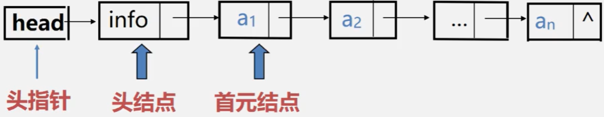
Header pointer: pointer to the first node in the linked list.
Head node: a node attached before the first node of the linked list.
First element node: refers to the node where the first data element a1 is stored in the linked list.
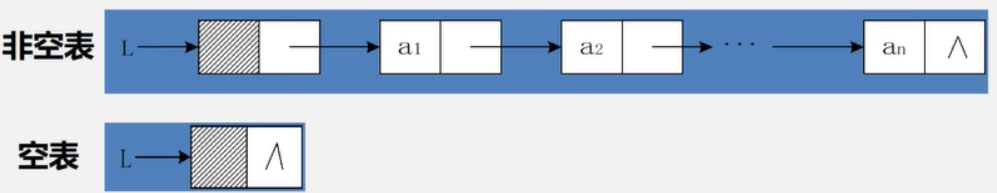
Schematic diagram of two forms of storage structure of linked list
① No lead node
② Leading node
discuss
1. How to represent an empty table?
① when there is no header node, if the header pointer is empty, it indicates an empty table.
② when there is a header node, when the pointer field of the header node is empty, it indicates an empty table.
2. What are the advantages of setting header nodes in the linked list?
① facilitate the processing of initial element nodes:
The address of the initial node is saved in the pointer field of the head node, so the operation at the first position of the linked list is consistent with other positions, and no special processing is required.
② facilitate the unified processing of empty and non empty tables:
No matter whether the linked list is empty or not, the head pointer refers to the non null pointer to the head node, so the processing of empty table and non empty table is unified.
3. What is installed in the data field of the header node?
The data field of the head node can be empty or store additional information such as the length of the linear table, but this node cannot be included in the length value of the linked list.
Characteristics of linked list (linked storage structure)
① the location of nodes in the memory is arbitrary, that is, logically adjacent data elements are not necessarily adjacent physically.
② when accessing, you can only enter the linked list through the header pointer, and scan the other nodes backward through the pointer field of each node, so the time spent looking for the first node and the last node is different.
※ this method of storing elements is called sequential storage method.

Single linked list
Definition and representation of single linked list
Single linked list of leading nodes
The single linked list is uniquely determined by the header, so the single linked list can be named after the head pointer. If the head pointer name is l, the linked list is called L.
Storage structure of single linked list
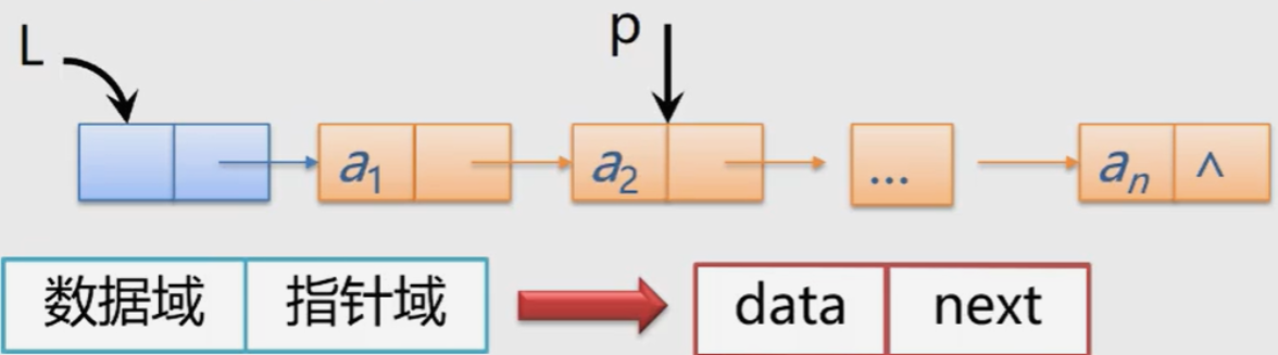
typedef struct Lnode{  //Declare the type of the node and the pointer type to the node
    ElemType data;  //A node is a data field
    struct Lnode *next;  //Pointer field of node
}Lnode, *LinkList;  //LinkList is the pointer type to the structure Lnode
LinkList L; //Define linked list L
Lnode *p; /*or*/ LinkList p;  //Define node pointer p
Main algorithm
Algorithm 1: initialization of single linked list (single linked list of leading node)
※ that is, construct an empty table
Algorithm steps:
① generate a new node as the head node, and point to the head node with the head pointer L.
② set the pointer field of the header node to null.
Status InitLIst_L(LinkList &L) {
	L = new LNode; //Or L = (LinkList)malloc(sizeof(LNode));
    L->next = NULL;
    return Ok;
}
Algorithm 2: judge whether the linked list is empty
Empty list: a linked list without elements is called an empty linked list (the head pointer and the head node are still there)
Algorithm idea: judge whether the pointer field of the header node is empty
int ListEmpty(LinkList L) {
    if(L->next)
        return 0;  //Non empty
    else
        return 1;
}
Algorithm 3: destruction of single linked list: the linked list does not exist after destruction
Algorithm idea: start from the pointer and release all nodes in turn.
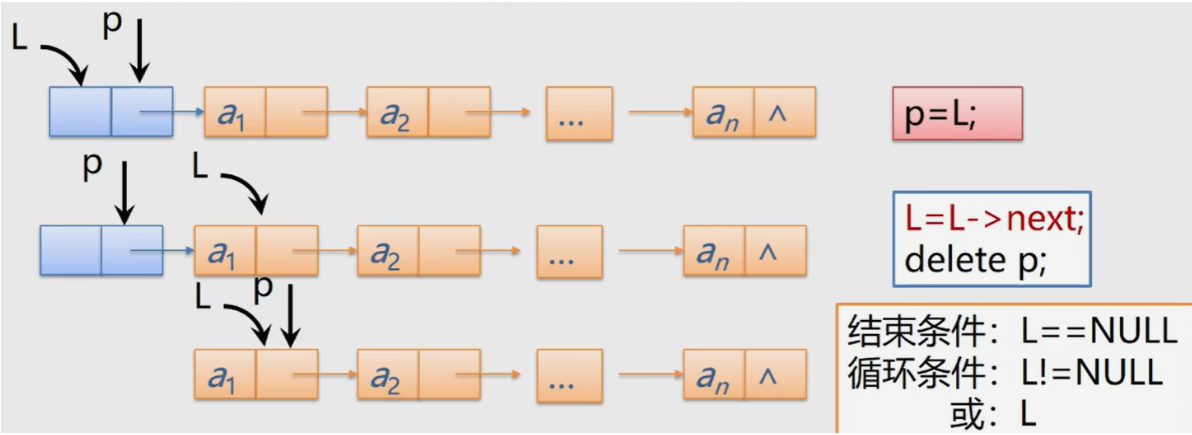
Status DestroyList_L(LinkList &L) { //Destroy single linked list L
    Lnode *p; // Or LinkList p
    while(L) {
        p = L;
        L = L->next;
        delete p;
    }
}
Algorithm 4: empty linked list
That is: the linked list still exists, but there are no elements in the linked list, so it becomes an empty linked list (the head pointer and head node are still there).
Algorithm idea: release all nodes in turn, and set the pointer field of the head node to null.
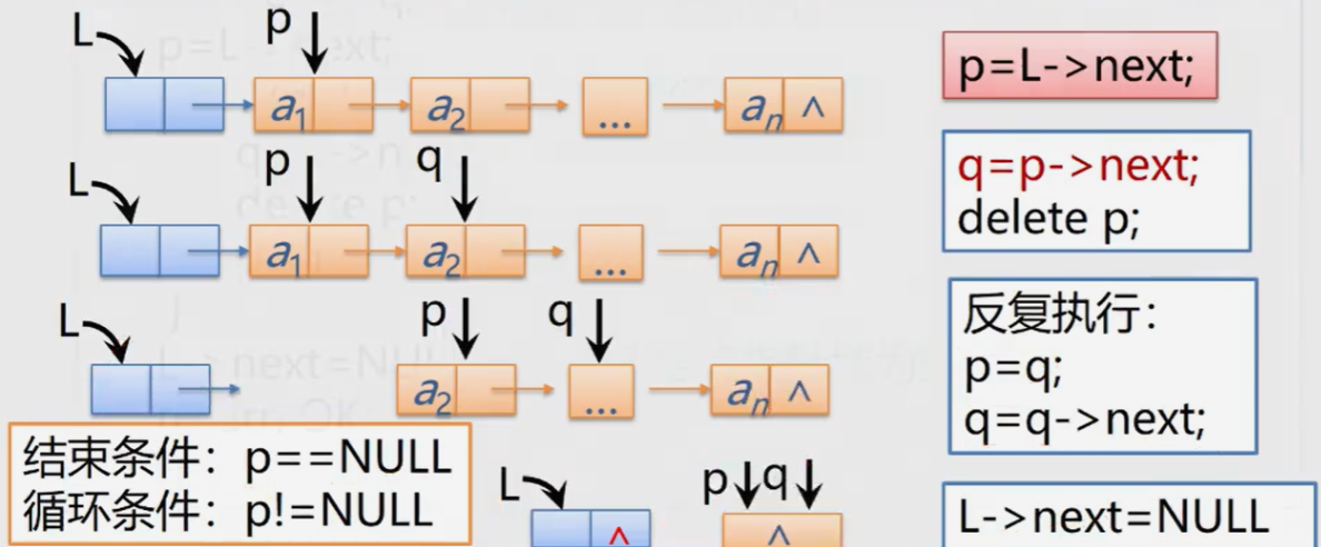
Status ClearList(LinkList &L){  //Reset L to empty table
    Lnode *p, *q;  //Or LinkList p,q;
    p = L->next;
    while(p) {  //It's not at the end of the watch
        q = p->next;
        delete p;
        p = q;
    }
    L->next = NULL;
    return OK;  //The header node pointer field is null
}
Algorithm 5: find the length of single linked list
Algorithm idea: start from the initial node and count all nodes in turn.
int ListLength_L(LinkList L) {  //Returns the number of data elements in L
    LinkList p;
    p = L->next;  //p points to the first node
    i = 0;
    while(p){  //Traverse the single linked list and count the number of nodes
        i++;
        p = p->next;
    }
    return i;
}
Algorithm 6: value - take the content of the ith element in the single linked list
Idea: starting from the head pointer of the linked list, search down the chain domain next node by node until the i-th node is searched. Therefore, the linked list is not a random storage structure.
Algorithm steps:
1. Scan in the chain from the first node (L - > next), point to the currently scanned node with pointer P, and the initial value of P is p = L - > next.
2.j is used as a counter to accumulate the number of nodes currently scanned, and the initial value of j is 1.
3. When p points to the next node scanned, the counter j increases by 1.
4. When j==i, the node p refers to is the ith node to be found.
Status GetElem_L(LinkList L, int i, ElemType &e){ //Get the content of a data element in linear table L and return it through variable e
    p = L->next; j = 1;  //initialization
    if(!p || j > i)   //The ith element does not exist
        return error;
    while(p && j < i){  //Scan backward until p points to the ith element or p is empty
        p = p->next;
        j++
    }
    e = p->data;  //Take the i th element
    return OK;
}
Algorithm 7: search by value -- obtain the location (address) of the number according to the specified data
Algorithm steps:
1. From the first node, compare with e in turn.
2. If a data element whose value is equal to e is found, its "position" or address in the linked list is returned.
3. If no element whose value is equal to e is found throughout the linked list, 0 or NULL is returned.
Lnode *LocateElem_L(LinkList L, Elemtype e){
    //Find the data element with the value e in the linear table L
    //If found, the address of the data element with e in the L value is returned. If the search fails, NULL is returned
    p = L->next;
    while(p && p->data != e)
        p = p->next;
    return p
}
Algorithm 8: search by value - obtain the serial number of the data location according to the specified data
//Find the position sequence number of the data element with the value e in the linear table L
int LocateElem_L(LinkList L, Elemtype e){
    //Returns the position sequence number of the data element with e in L. if the search fails, it returns 0
    p = L->next; j = 1;
        while(p && p->data != e)
        {
            p = p->next;
            j++;
        }
    if(p)
        return j;
    else return 0;
}
Time complexity O(n)
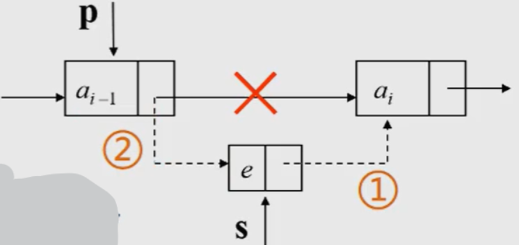
Algorithm 9: inserting nodes
Algorithm steps:
1. First find the storage location p of ai-1.
2. Generate a new node s with data field e.
3. Insert new node: ① the pointer field of the new node points to node a s - > next = P - > next
② the pointer field of node ai-1 points to the new node p - > next = s
//Insert the data element e before the ith element in L
Status LintInsert_L(LinkList &L, int i, ElemType e){
    p = L; j = 0;
    while(p && j < i-1){  //Find the i-1 node, and p points to the i-1 node
        p = p->next;
        j++;
    }
    if(!p || j > i-1)
        return error;  //If i is greater than + 1 or less than 1, the insertion position is illegal
    s = new LNode;  //Generate new node s
    s->data = e;  //Set the data field of node s to e
    s->next = p->next;  //Insert node s into L
    p->next = s;
    return OK;
}
The time complexity is O(1), and the need to find is O(n)
Algorithm 10: delete - delete the ith node
Algorithm steps: 1 First, find the storage location p of ai-1 and save the value of ai to be deleted.
2. Make p - > next point to ai+1
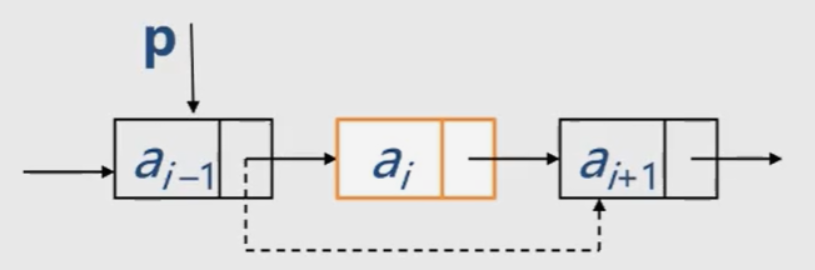
Core steps: P - > next = P - > next - > next
//Delete the ith data element in linear table L
Status ListDelete_L(LinkList &L, int i, ElemType &e){
    p = L; j = 0; q;
    while(p->next && j<i-1){ //Find the ith node and point p to its precursor
        p = p->next;
        j++;
    }
    if(!(p->next) || j > i-1)  //Unreasonable deletion position
        return error;
    q = p-next;  //Temporarily save the address of the deleted node for release
    p->next = q->next;  //Change the pointer field of the precursor node of the deleted node
    e = q->data;  //Save delete node data field
    delete q; //Free up space for deleting nodes
    return OK;
}
The time complexity is O(1), and the need to find is O(n)
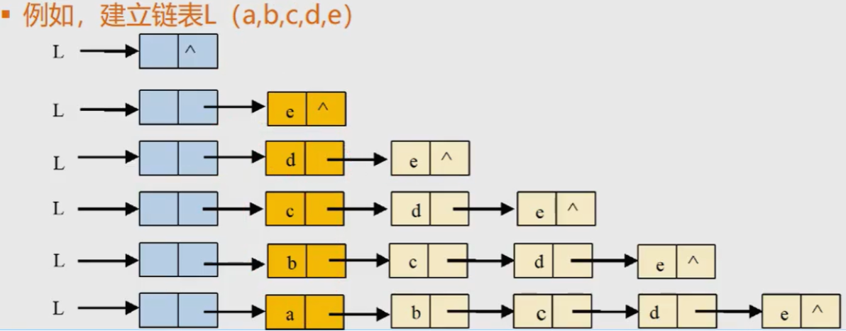
Algorithm 11: establish a single linked list: head insertion - elements are inserted into the head of the linked list, also known as pre insertion
Algorithm steps: 1 Start with an empty table and read data repeatedly.
2. Generate a new node and store the read data in the number field of the new node.
3. Starting from the last node, insert each node into the front end of the linked list in turn
void CreateList_H(LinkList &L, int n){
    L = new LNode;
    L->next = NULL;  //First establish a single linked list of leading nodes
    for(i = n; i > 0; --i){
        p = new LNode;  //Generate a new node p = (LNode*)malloc(sizeof(LNode));
        cin >> p->data;  //Enter the element value scanf (& P - > data);
        p->next = L->next; //Insert into header
        L->next = p;
    }
}
Time complexity O(n)
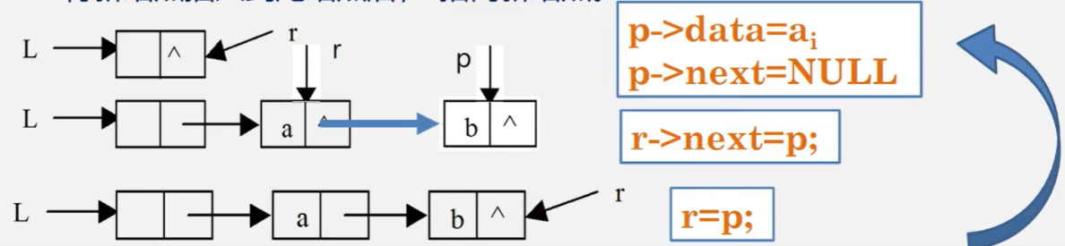
Algorithm 12: establish a single linked list: tail interpolation - elements are inserted at the tail of the linked list, also known as post interpolation
Algorithm steps: 1 Starting from an empty list L, insert new nodes one by one into the tail of the linked list, and the tail pointer r points to the tail node of the linked list.
2. Initially, r and L refer to the head node. Every time a data element is read in, a new node is applied. After the new node is inserted into the tail node, r points to the new node.
//Enter the values of n elements in the positive bit order to establish a single linked list L with header nodes
void CreateList_R(LinkList &L, int n){
    L = new LNode;
    L->next = NULL;
    r = L;  //The tail pointer r points to the head node
    for(i = 0; i < n; i++){
        p = new LNode;  //Generate a new node and enter the element value
        cin >> p->data;
        p->next = NULL;
        r->next = p;  //Insert to footer
        r = p;  //r points to the new tail node
    }
}
Time complexity O(n)
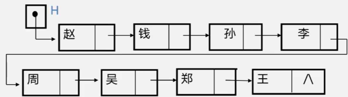
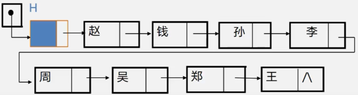
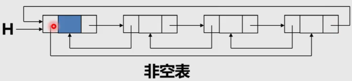
Circular linked list
Circular linked list: it is a linked list with head and tail connected (that is, the pointer field of the last node in the list points to the head node, and the whole linked list forms a ring).
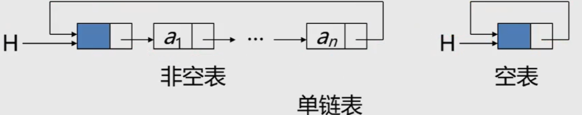
Advantages: starting from any node in the table, you can find other nodes in the table.
Note: since there is no NULL pointer in the circular linked list, when traversal is involved, the termination condition will no longer judge whether p or p - > next is NULL as in the non circular linked list, but whether they are equal to the header pointer. (p! = l or p - > next! = L)
Merging of circular linked list with tail pointer (merging Tb after Ta)
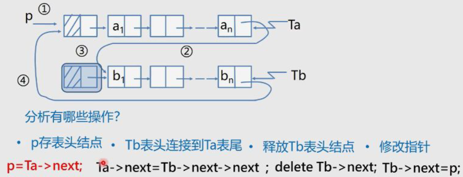
LinkList Connect(LinkList Ta, LinkList Tb){
    //Suppose that Ta and Tb are non empty single cycle linked lists
    p = Ta->next;  //① p save header node
    Ta->next = Tb->next->next;  //② Tb header connected to Ta footer
    delete Tb->next;  //③ Release Tb header node
    Tb->next = p;  //④ Modify pointer
    return Tb;
}
Time complexity O(1)
Bidirectional linked list
Why discuss two-way linked lists?
The node of the single linked list - > has a pointer field indicating the successor - > it is convenient to find the successor node; That is, the execution time of finding the successor node of a node is O(1).
——>Pointer field without indicating precursor - > it is difficult to find precursor node: start from the header; That is, the execution time of finding the precursor node of a node is O(n).
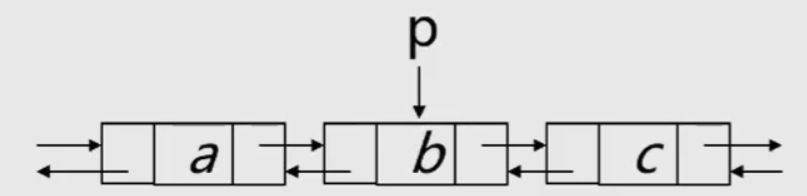
Bidirectional linked list: add a pointer field prior to its direct precursor in each node of the single linked list, so that chains with two different directions are formed in the linked list, so it is called bidirectional linked list.
Structure definition of bidirectional linked list
typedef struct DulNode{
    Elemtpye data;
    struct DulNode *prior, *next;
}DulNode, *DuLinkList;
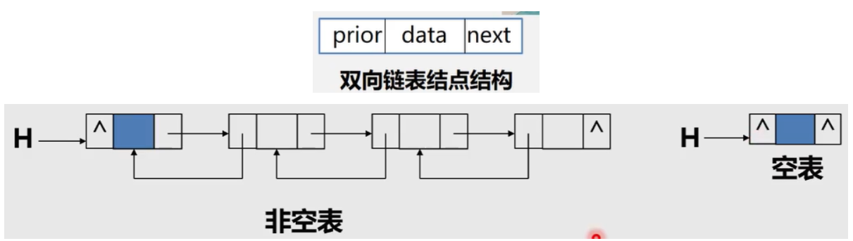
Bidirectional circular linked list
Similar to a single linked circular table, a two-way linked list can also have a circular table.
That is, let the precursor pointer of the head node point to the last node of the linked list; Let the subsequent pointer of the last node point to the head node.
Characteristics of bidirectional linked list
Symmetry of bidirectional linked list structure (set pointer p to a node)
That is: P - > priority - > next = P = P - > next - > priority
In a two-way linked list, some operations (such as ListLength, GetElem, etc.) only involve pointers in one direction, so their algorithm is the same as that of a linear linked list. However, when inserting and deleting, you need to modify the pointers in both directions at the same time, and the time complexity of both operations is O(n).
Algorithm 1: insertion of bidirectional linked list
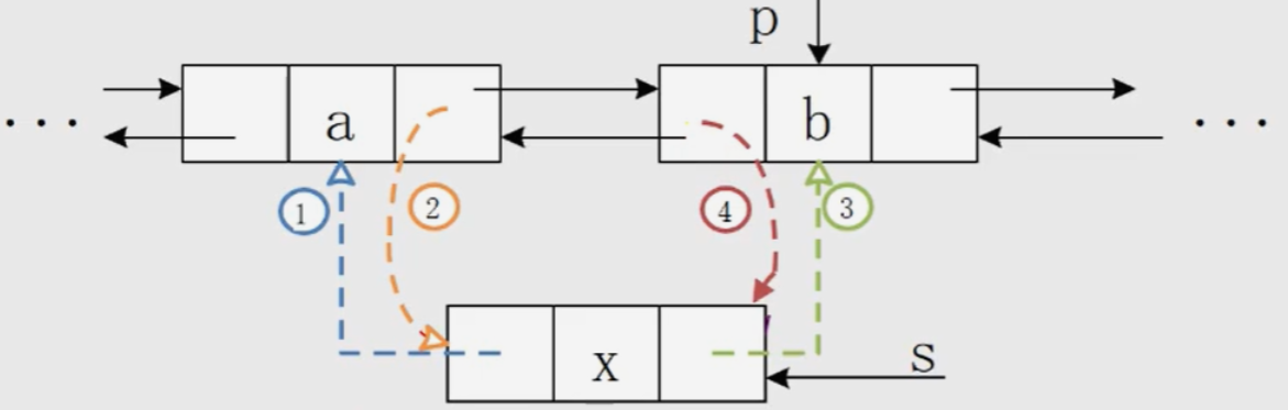
Core steps:
-
s->prior = p->prior
-
p->prior->next = s
-
s->next = p;
-
p->prior = s;
void ListInsert_Dul(DuLinkList &L, int i, ElemType e){
    //Insert element e before the ith position in the bidirectional circular linked list L of the leading node
    if(!(p = GetElemP_DuL(L,i)))  //Judge whether the insertion position is reasonable
        return error;
    s = new DULNode;
    s->data = e;
    s->prior = p->prior;
    p->prior->next = s;
    s->next = p;
    p->prior = s;
    return OK;
}
Time complexity O(n)
Algorithm 2: deletion of bidirectional linked list
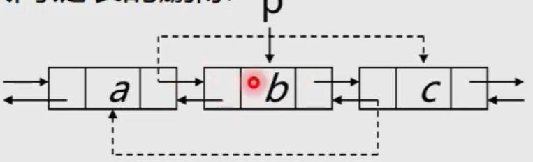
Core steps:
1.p->prior->next = p->next;
2.p->next->prior = p->prior;
void ListDelete_DuL(DuLink &L, int i, ElemType &e){
    //Delete the ith element of the two-way linked list L of the leading node and return it with e
    if(!(p = GetElemP_DuL(L,i)))  //Judge whether the deletion position is reasonable
        return error;
    e = p->data;
    p->prior->next = p->next;
    p->next->prior = p->prior;
    free(p);
    return OK;
}
Time complexity O(n)
Time efficiency comparison of single linked list, circular linked list and two-way linked list
| Find header node (initial node) | Lookup table footer | Find the precursor node of node * p | |
|---|---|---|---|
| Single linked list L of leading node | L - > next time complexity O(1) | Traverse backward successively from L - > next, with time complexity O(n) | Its precursor cannot be found through p - > next |
| The leading node is a circular single linked list with only head pointer L | L - > next time complexity O(1) | Traverse backward successively from L - > next, with time complexity O(n) | The precursor can be found through p - > next, and the time complexity is O(n) |
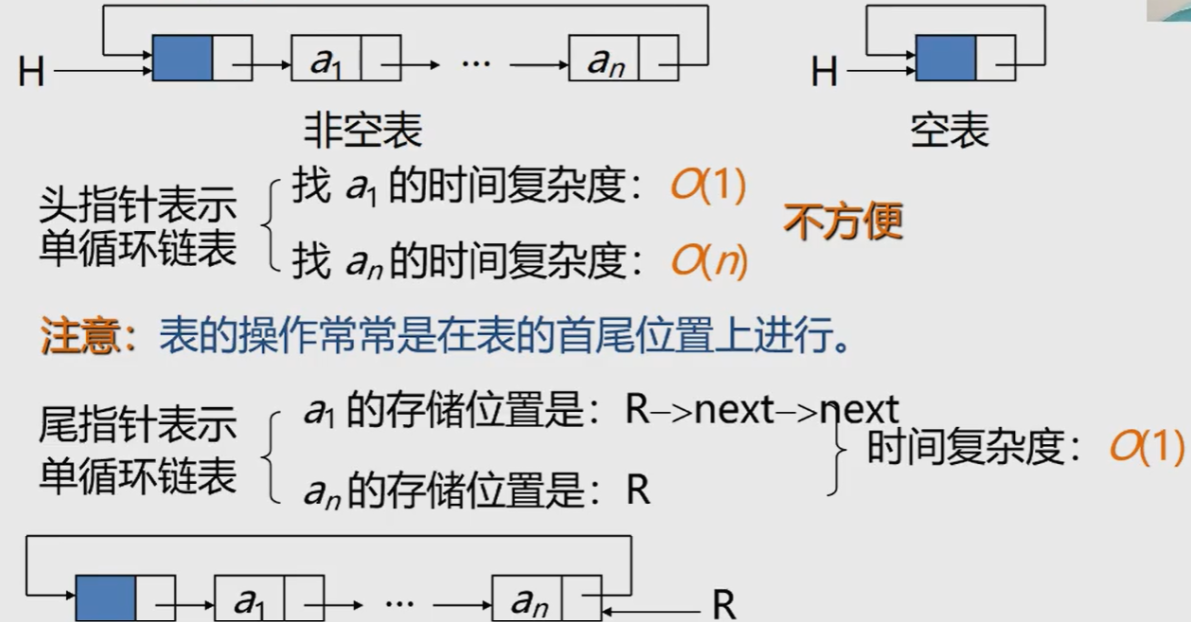
| Cyclic single linked list with only tail pointer R at the leading node | R - > next time complexity O(1) | R. Traverse backward successively from L - > next, with time complexity O(1) | The precursor can be found through p - > next, and the time complexity is O(n) |
| Bidirectional circular linked list L of the leading node | L - > next time complexity O(1) | L - > prior, time complexity O(1) | P - > prior, time complexity O(1) |
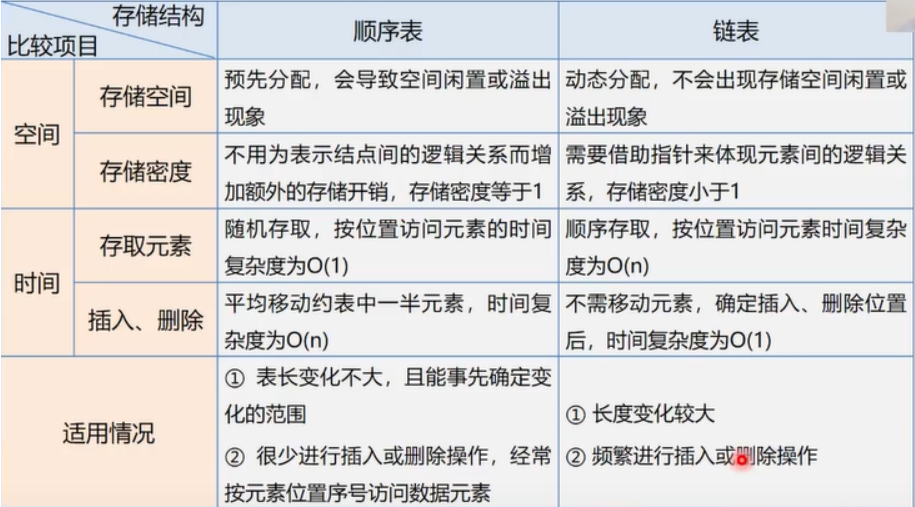
Comparison of sequential list and linked list
Advantages of chained storage structure:
① node space can be dynamically applied and released;
② the logical order of data elements is indicated by the pointer of the node. There is no need to move the elements during insertion and deletion.
Disadvantages of chain storage structure:
① the storage density is small, and the pointer field of each node needs to occupy additional storage space. When the data field of each node occupies few bytes, the proportion of pointer field in storage space is very large.
② the chain storage structure is a non random access structure. The operation of any node must find the node from the beginning pointer according to the pointer chain, which increases the complexity of the algorithm.
Storage density
Storage density refers to the ratio of the storage capacity of node data itself to the storage capacity of the whole node structure, that is:
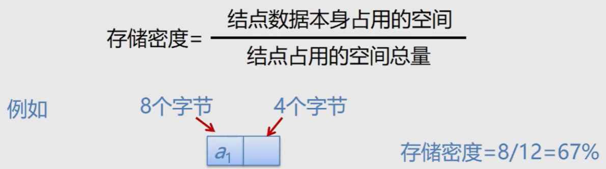
Generally, the higher the storage density, the higher the utilization of storage space. Obviously, the storage density of the sequential list is 1 (100%), while the storage density of the linked list is less than 1.
Application of linear table
Merging of linear tables
Problem Description:
Assuming that two linear tables La and Lb are used to represent two sets A and B respectively, A new set A = A U B is required
La = (7, 5, 3, 11) Lb = (2, 6, 3) ==> La = (7, 5, 3, 11, 2, 6)
Algorithm steps:
Take out each element in Lb in turn and perform the following operations:
1. Find the element in La
2. If not, insert it at the end of La
void union(List &La, List Lb){
    La_len = ListLength(La);
    Lb_len = ListLength(Lb);
    for(i = 1; i <= Lb_len; i++){
        GetElem(Lb, i, e);
        if(!LocateElem(La, e))
            ListInsert(&La, ++La_len, e);
    }
}//Time complexity: O(ListLength(La) * ListLength(Lb))
Consolidation of ordered tables
Problem Description:
It is known that the data elements in the linear tables La and Lb are arranged in non decreasing order. Now it is required to merge La and Lb into a new linear table Lc, and the data elements in Lc are still arranged in non decreasing order.
La = (1, 7, 8) Lb = (2, 4, 6, 8, 10, 11) ==> Lc = (1, 2, 4, 6, 7, 8, 8, 10, 11)
Algorithm steps:
1. Create an empty table Lc
2. Successively "extract" the node with smaller element value from La or Lb and insert it into the last of Lc table until one of the tables becomes empty
3. Continue to insert the remaining nodes of one of the tables La or Lb at the end of the Lc table
//Implementation with sequence table
void MergeList_Sq(SqList LA, SqList LB, SqList &LC){
    pa = LA.elem;
    pb = LB.elem;  //The initial values of pointers pa and pb point to the first element of the two tables respectively
    LC.length = LA.length + LB.length;  //The length of the new table is the sum of the lengths of the two tables to be merged
    LC.elem = new ElemType[LC.length];  //Allocate an array space for the merged new table
    pc = LC.elem;  //The pointer pc points to the first element of the new table
    pa_last  = LA.elem + LA.length-1;  //Pointer pa_last points to the last element of the LA table
    pb_last  = LB.elem + LB.length-1;  //Pointer pb_last points to the last element of the LB table
    while(pa <= pa_last && pb <= pb_last){  //Neither table is empty
        if(*pa <= *pb)   //"Pick" the nodes with smaller values in the two tables in turn
            *pc++ = *pa++;
        else *pc++ = *pb++;
    }
    while(pa <= pa_last)  //LB table has reached the end of the table. Add the remaining elements in LA to LC
        *pc++ = *pa++;
    while(pb <= pb_last)  //LA table has reached the end of the table. Add the remaining elements in LB to LC
        *pc++ = *pb++;
}//Time complexity: O(ListLength(LA) * ListLength(LB))
 //Space complexity: O(ListLength(LA) * ListLength(LB))
Using linked list
void MergeList_Sq(SqList La, SqList Lb, SqList &Lc){
    pa = La->next;
    pb = Lb->next;
    pc = Lc = La;  //The head node of La is used as the head node of Lc
    while(pa && pb){
        if(pa->data <= pb->data){
            pc->next = pa;
            pc = pa;
            pa = pa->next;
        }else{
            pc->next = pb;
            pc = pb;
            pb = pb->next;
        }
    }
    pc->next = pa?pa:pb; //Insert remaining segments
    delete Lb;  //Release the header node of Lb
}//Time complexity: O(ListLength(La) * ListLength(Lb))