Recursive Preface
I believe you all know very well about Recursion, so we won't elaborate here. For details, please refer to the recursive function in the Python function chapter.
The three laws of recursion are as follows:
- Recursive algorithms must have a basic end condition
- Recursive algorithms must be able to change the size of the problem
- The recursive algorithm must call itself
Divide and conquer strategy
Divide and conquer strategy means that a large-scale problem is decomposed into smaller same problems. After continuous decomposition, the scale of the problem is small enough to be solved in a very simple and direct way, or a problem is divided into different parts, solved by division and ruled by division.
The divide and conquer strategy generally goes through three steps:
- Partitioning: this step involves breaking down the problem into smaller subproblems. The subproblem should represent part of the original problem. This step usually uses recursive method to divide the problem until no sub problem can be further divided. At this stage, the subproblem essentially becomes an atom, but it still represents part of the actual problem
- Solution: many smaller sub problems need to be solved in this step. Generally, at this level, the problem is considered to be "solved" by itself.
- Merging: when smaller subproblems are solved, this stage will begin to combine them recursively until they are merged into the solution of the original problem.
Binary conversion
In the previous linear structure (stack), we have realized a conversion of hexadecimal to hexadecimal. If we use recursive functions, the whole implementation process will become very simple.
As follows:
def baseConversion(n, base):
    digits = "0123456789ABCDEF"
    if n < base:
        return digits[n]
    return baseConversion(n // base, base) + digits[n % base]

if __name__ == "__main__":
    print(baseConversion(101, 2))
    print(baseConversion(101, 8))
    print(baseConversion(101, 16))

# 1100101
# 145
# 65
Hanoi
The Hanoi Tower problem was proposed by the French mathematician Edward Lucas in 1883.
He was inspired by a legend that a Hindu temple gave the puzzle to a young priest. At the beginning, the priest was given three poles and a pile of 64 gold discs, each smaller than the one below it.
The priest's task is to transfer all 64 plates from one of the three rods to the other.
There are two important constraints:
- Only one plate can be moved at a time
- Larger plates cannot be placed on top of smaller plates.
The priest kept moving a plate every second day and night. It is said that when he finished his work, the temple would turn into dust and the world would disappear.
The rules of the game are shown in the figure below:

How to solve it by recursion? We first analyze the rules of the game of Hanoi Tower itself.
As can be seen from the above figure, the discs of models s and m must be located on the pole B through the pole C. We can regard any number of discs other than the largest as a whole group, while the largest disc is divided into a group separately. The discs are divided into two groups in total, and they are divided according to groups when moving:
The algorithm is as follows, so it can be divided into three steps:
- Move n-1 discs from column A through C to B, but omit the step to C and go directly to B
- Move the n th disc (the largest disc) from A to C
- Move n-1 discs from B through A to C, but omit the step to A and go directly to C
The code is as follows. First solve according to three discs:
def hanoi(n, a, b, c):
    if n:
        # From a to c to b
        hanoi(n - 1, a, c, b)
        # From a to c
        print("moving from %s to %s" % (a, c))
        # From b through a to c
        hanoi(n - 1, b, a, c)


if __name__ == "__main__":
    hanoi(3, "A", "B", "C")

# moving from A to C
# moving from A to B
# moving from C to B
# moving from A to C
# moving from B to A
# moving from B to C
# moving from A to C
greedy strategy
Greedy algorithm (also known as greedy algorithm) means that when solving a problem, it always makes the best choice at present.
In other words, without considering the overall optimization, the algorithm obtains the local optimal solution in a sense.
Greedy algorithm can not get the overall optimal solution for all problems. The key is the choice of greedy strategy.
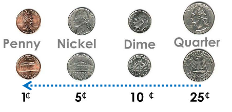
Change-Making Problem
Suppose you program a vending machine manufacturer. The vending machine should give customers the minimum number of coins each time;
Suppose a customer puts in a $1 note and buys it ȼ 37 (cents) things, looking for ȼ 63, then the minimum quantity is: 2 quarter s( ȼ 25) 1 dime( ȼ 10) And 3 penny( ȼ 1) , a total of six.
People will adopt various strategies to solve these problems, such as the most intuitive "greedy strategy". Generally, we do this:
- Start with the coin with the largest denomination and use as few coins as possible to find as much balance as possible until the largest one cannot be found
- Go to the next coin with the largest denomination until you reach penny( ȼ 1) So far.
Because we try to solve the biggest part of the problem every time. Corresponding to the coin exchange problem, we quickly reduce the change face value with the largest number of coins with the largest face value every time. This is the greedy strategy. The code is as follows. You can try to rewrite it into recursive implementation:
def findCoins(coinValueList, change):
    """
    :param coinValueList: Incoming coin system
    :param change: Pass in the coin to be recovered
    :return: How much information is returned
    """
    minCoins = ""
    for coin in coinValueList[::-1]:
        # If the money to be found is greater than the maximum face value, the algorithm starts
        if change >= coin:
            # How many coins of the largest denomination can I find at most?
            n = int(change // coin)
            # What's the maximum change?
            amount = n * coin
            # How much money is missing? Get ready for the next round
            change -= amount
            # How many coins have you found this time? How many yuan is the coin
            minCoins += "%s Pieces%s Yuan coin\n" % (n, coin)
    return minCoins


if __name__ == '__main__':
    print(findCoins([1, 5, 10, 25], 63))

# Two 25 yuan coins
# One 10 yuan coin
# Three one dollar coins
The recursive implementation is as follows:
def findCoins(coinValueList, change):
    minCoins = ""
    coin = coinValueList[-1]

    if change >= coin:
        n = int(change // coin)
        amount = n * coin
        change -= amount
        minCoins += "%s Pieces%s Yuan coin\n" % (n, coin)
        if change == 0:
            return minCoins
    return findCoins(coinValueList[:-1], change=change) + minCoins


if __name__ == '__main__':
    print(findCoins([1, 5, 10, 25], 63))

# Three one dollar coins
# One 10 yuan coin
# Two 25 yuan coins
dynamic programming
The dynamic programming method is similar to the divide and conquer method, which decomposes the problem into smaller possible subproblems, but different from the divide and conquer method, these subproblems are not solved independently. On the contrary, the results of these smaller subproblems will be remembered and used for similar or overlapping subproblems.
Using dynamic programming where we encounter problems, we can divide these problems into similar sub problems so that their results can be reused.
In most cases, the algorithm is often used for optimization. Before solving the existing subproblem, the dynamic algorithm will try to check the results of the previously solved subproblem. The solutions of sub problems are combined to obtain the best solution.
So we can say:
- The problem should be able to be divided into smaller overlapping subproblems
- The optimal solution can be achieved by using the optimal solution of a smaller problem
- Dynamic algorithms use memory
Elbonia's strange coin system
”"Greedy strategy" solves the problem of change and performs well under the coin system of US dollar or other currencies, but if your boss decides to export the vending machine to Elbonia, things will be a little complicated.
Elbonia is a country invented in the comic series Dilbert
In addition to the above three denominations, there is one in this strange country[ ȼ 21] coins!
According to the "greedy strategy", in Elbonia, ȼ 63 or the original six coins:
ȼ63 =ȼ25*2+ȼ10*1+ȼ1*3
But in fact, the optimal solution is three denominations ȼ 21 coins!
ȼ63 =ȼ21*3
So... The greedy strategy failed.
Routine solution
Let's find a way to find the optimal solution and give up the greedy strategy.
Because whether the greedy strategy is effective depends on the specific coin system. For example, in Elbonia's monetary system, the greedy strategy fails.
The first is to determine the basic ending conditions. The simplest and direct case of coin exchange is that the face value of the change to be exchanged is exactly equal to a certain coin, such as 25 cents. The answer is a coin!
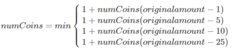
The second is to reduce the scale of the problem. We should try once for each coin, such as the dollar coin system:
- After subtracting 1 penny from the change, find the minimum number of coins to exchange (recursively call itself)
- Find the minimum number of coins to change after subtracting 5 cents from the change
- After the change minus 10 cents (dime), find the minimum number of coins to exchange
- After the change minus 25 cents, find the minimum number of coins to change
- Select the smallest of the above four items
The code implementation is as follows:
#! /usr/local/bin/python3
# -*- coding:utf-8 -*-

def recMC(coinValueList, change):
    minCoins = change
    if change in coinValueList:
        return 1
    else:
        for i in [c for c in coinValueList if c <= change]:
            numCoins = 1 + recMC(coinValueList, change - i)
            if numCoins < minCoins:
                minCoins = numCoins
    return minCoins


if __name__ == '__main__':
    print(recMC([1, 5, 10, 25], 63))
For the 63 cent coin exchange problem, 67716925 recursive calls are required.
In this implementation scheme, I ran for more than 40 seconds, because there are a large number of sub recursive repeated calculations.
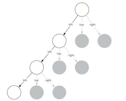
For example, the change of 15 points appeared three times! It needs 52 recursive calls to be finally solved. The figure below is only a corner of recursion:

Optimization scheme
The key to the improvement of this recursive solution is to eliminate repeated calculation. We can use a table to save the calculated intermediate results. Before calculation, check the table to see whether it has been calculated. If it has been calculated, the function will not be run, so the function stack frame will not be generated, which greatly reduces the running time. This is dynamic programming.
Although this approach will increase the spatial complexity, it will greatly reduce the time complexity, that is, each subproblem will be solved only once.
Before recursive call, first look up whether there is an optimal solution for partial change in the table. If so, directly return the optimal solution without recursive call. If not, make recursive call.
The code implementation is as follows:
#! /usr/local/bin/python3
# -*- coding:utf-8 -*-

def recDC(coinValueList,change,knownResults):
    """
    :param coinValueList:
    :param change:
    :param knownResults: The result of saving the table (corresponding to the memo mode in the design mode), because we want to change 63, we can set it as a list with a width of 64
    """
    minCoins = change
    # Basic conditions for recursive end
    if change in coinValueList:
       # Record optimal solution
      knownResults[change] = 1
      return 1
    elif knownResults[change] > 0:
       # Look up the table successfully and use the optimal solution directly
      return knownResults[change]
    else:
       for i in [c for c in coinValueList if c <= change]:
         numCoins = 1 + recDC(coinValueList, change-i,
                              knownResults)
         if numCoins < minCoins:
            minCoins = numCoins
            # Find the optimal solution and record it in the table
            knownResults[change] = minCoins
    return minCoins

if __name__ == '__main__':
    print(recDC([1,5,10,25],63,[0]*64))
Now call again, and it only takes a few tenths of a second to get the result.
Python built-in library functools @ lrc_chace also implements this caching function, but the decorator uses dictionary storage cache, so the fixed parameters and keyword parameters of the decorated function must be hashable.
As shown below, instead of writing dynamic programming by yourself, you can call the decorator directly. You only need to change the currency system input from list to tuple:
#! /usr/local/bin/python3
# -*- coding:utf-8 -*-

import functools


@functools.lru_cache(maxsize=63)
def recMC(coinValueList, change):
    minCoins = change
    if change in coinValueList:
        return 1
    else:
        for i in [c for c in coinValueList if c <= change]:
            numCoins = 1 + recMC(coinValueList, change - i)
            if numCoins < minCoins:
                minCoins = numCoins
    return minCoins


if __name__ == '__main__':
    print(recMC((1, 5, 10, 25), 63))
    # list can't be hash, just change it to tuple
Recursive visualization
turtle module
This is a Python built-in module that can be called at any time to simulate the footprints left by a turtle crawling on the beach based on the creativity of LOGO language.
Here are some basic methods:
| method | describe |
|---|---|
| turtle.Turtle() | Instantiate object |
| hideturtle() | Make the tortoise invisible, leaving only footprints |
| forward() | The tortoise moves forward (head to the East) |
| backward() | The tortoise moves backward (head West) |
| left() | The tortoise turned to the left |
| right() | The tortoise turned to the right |
| penup() | Lift the brush |
| pendown() | Put down the brush |
| pensize() | Pen width |
| pencolor() | Pen color |
| turtle.done() | Do not close after painting |
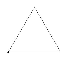
Draw a triangle:
import turtle
import time


def triangle():
    t = turtle.Turtle()
    t.forward(200)
    t.right(60)
    t.backward(200)
    t.left(120)
    t.backward(200)


if __name__ == '__main__':
    triangle()
    time.sleep(5)
Self similar recursive graph
Fractal is a new discipline initiated by Mandelbrot in 1975.
Its concept is: "a rough or fragmentary geometry can be divided into several parts, and each part (at least approximately) is the shape after overall reduction", that is, it has self similar properties.
There are many self similar recursive graphics in nature, such as snowflakes, branches and so on:

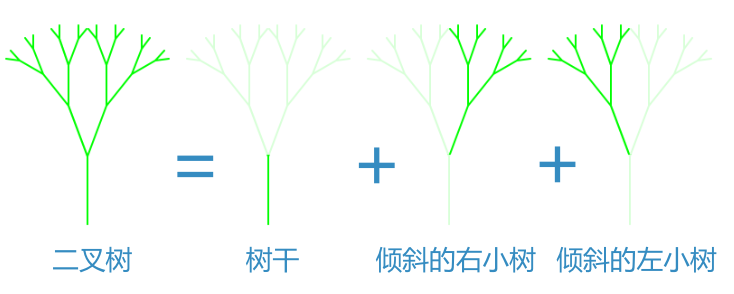
Fractal tree
We can use recursion to draw a binary fractal tree and divide the tree into three parts: trunk, small tree on the left and small tree on the right.
After decomposition, it just conforms to the definition of recursion: the call to itself.
The code is as follows:
import turtle


def tree(branch_len: int, t: turtle.Turtle) -> None:
    # Recursive end condition, the trunk cannot be too short
    if branch_len > 5:
        # Draw trunk
        t.forward(branch_len)
        # Tilt right 20 degrees
        t.right(20)
        # Recursion, draw right decimal, trunk - 15
        tree(branch_len - 15, t)
        # Tilt left by 40 degrees, i.e. tilt left by 20 degrees after straightening
        t.left(40)
        # Recursion, draw left decimal, trunk - 15
        tree(branch_len - 15, t)
        # Right tilt 20 degrees, i.e. return to normal
        t.right(20)
        # The turtle returned to its original position
        t.backward(branch_len)


if __name__ == '__main__':
    t = turtle.Turtle()
    # Turn around, due north
    t.left(90)
    # pen-up
    t.penup()
    # Lift up 100 px
    t.backward(100)
    # Write
    t.pendown()
    # Pen width: 2, color: Green
    t.pencolor("green")
    t.pensize(2)
    # Start drawing a trunk with a length of 75
    tree(75, t)
    # Make the tortoise invisible
    t.hideturtle()
    # Do not close on exit
    turtle.done()
Effect demonstration:
Shelbins triangle
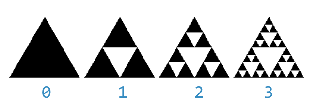
The sherbins triangle Sierpinski is a type structure.
Create a triangle, and then divide the triangle into three parts each time. Dig it unlimited. Finally, the area of the triangle will become 0 and the perimeter will become infinite. It is a fractional dimension (about 1.585 dimensions) structure between one and two dimensions.
According to the characteristics of self similarity, the shelpinski triangle is made up of three shelpinski triangles whose sizes are halved according to the product shape.
Because we can't really make the shelbinsky triangle (degree - > ∞), we can only make the approximate graph of degree limited.
In the case of limited degree, the triangle with degree=n is made up of three triangles with degree=n-1 stacked according to the shape of goods. At the same time, the side length of the three triangles with degree=n-1 is half of that of the triangle with degree=n (the scale is reduced).
When degree=0, it is an equilateral triangle, which is the basic end condition of recursion.
The code is as follows. Those interested can study it carefully:
import turtle


def drawTriangle(points, color, myTurtle):
    myTurtle.fillcolor(color)
    myTurtle.up()
    myTurtle.goto(points[0][0], points[0][1])
    myTurtle.down()
    myTurtle.begin_fill()
    myTurtle.goto(points[1][0], points[1][1])
    myTurtle.goto(points[2][0], points[2][1])
    myTurtle.goto(points[0][0], points[0][1])
    myTurtle.end_fill()


def getMid(p1, p2):
    return ((p1[0] + p2[0]) / 2, (p1[1] + p2[1]) / 2)


def sierpinski(points, degree, myTurtle):
    colormap = ['blue', 'red', 'green', 'white', 'yellow',
                'violet', 'orange']
    drawTriangle(points, colormap[degree], myTurtle)
    if degree > 0:
        sierpinski([points[0],
                    getMid(points[0], points[1]),
                    getMid(points[0], points[2])],
                   degree - 1, myTurtle)
        sierpinski([points[1],
                    getMid(points[0], points[1]),
                    getMid(points[1], points[2])],
                   degree - 1, myTurtle)
        sierpinski([points[2],
                    getMid(points[2], points[1]),
                    getMid(points[0], points[2])],
                   degree - 1, myTurtle)


def main():
    myTurtle = turtle.Turtle()
    myWin = turtle.Screen()
    myPoints = [[-100, -50], [0, 100], [100, -50]]
    sierpinski(myPoints, 3, myTurtle)
    myWin.exitonclick()


if __name__ == '__main__':
    main()
Effect demonstration:
Drawing steps: