Stacking integration algorithm can be understood as a two-layer integration. The first layer contains multiple basic classifiers to provide the prediction results (meta features) to the second layer, while the classifier of the second layer is usually logistic regression. He takes the results of the first layer classifier as features to fit and output the prediction results.

1 Blending ensemble learning algorithm

Blending ensemble learning algorithm is a simplified version of Stacking ensemble algorithm.

1.1 algorithm flow

Algorithm flow of Blending integrated learning:

1. The data set is divided into training set and test_set, and then the training set is divided into training set and valid_set again. For example, if the data set with 10000 samples is divided into 80% training and 20% testing for the first time, then test_ The set has 2000 samples and the training data has 8000 samples. The 8000 samples are divided again for the second time, 70% as the training set and 30% as the test set, then train_set has 5600 samples and 2400 samples are valid_ set.
2. Then create the first layer of multi models, which can be homogeneous or heterogeneous. For example, in this layer, we use k SVM, or SVM, random forest and XGBoost.
3. Using train_ The multi model of the first layer is trained by set m o d e l A = { m o d e l 1 , m o d e l 2 , ... , m o d e l k } modelA=\{model_1,model_2,\dots,model_k\} modelA={model1, model2,..., modelk}, and then use these K models to predict the validity_ Set and test_set to get k groups of valid_predict and test_predict1 (each model predicts a set of results). here v a l i d _ p r e d i c t = { v a l i d _ p r e d i c t 1 , v a l i d _ p r e d i c t 2 , ... , v a l i d _ p r e d i c t k } t e s t _ p r e d i c t 1 = { t e s t _ p r e d i c t 1 ， t e s t _ p r e d i c t 2 , ... , t e s t _ p r e d i c t k } valid\_predict=\{valid\_predict_1,valid\_predict_2,\dots,valid\_predict_k\}\\ test\_predict1=\{test\_predict_1，test\_predict_2,\dots,test\_predict_k\} valid_predict={valid_predict1​,valid_predict2​,...,valid_predictk​}test_predict1={test_predict1​，test_predict2​,...,test_predictk​}
4. Create the model of the second layer and predict it with the first layer v a l i d _ p r e d i c t = { v a l i d _ p r e d i c t 1 , v a l i d _ p r e d i c t 2 , ... , v a l i d _ p r e d i c t k } valid\_predict=\{valid\_predict_1,valid\_predict_2,\dots,valid\_predict_k\} valid_predict={valid_predict1, valid_predict2,..., valid_predictk} as the training data of the second layer model, train to get the model modelB of the second layer, and then predict the training data of the first layer t e s t _ p r e d i c t 1 = { t e s t _ p r e d i c t 1 ， t e s t _ p r e d i c t 2 , ... , t e s t _ p r e d i c t k } test\_predict1=\{test\_predict_1，test\_predict_2,\dots,test\_predict_k\} test_predict1={test_predict1, test_predict2,..., test_predictk} to obtain the final prediction result test_ predict.

• Advantages of Blending algorithm:
  The implementation is simple and rough without much theoretical analysis.
• Disadvantages of Blending algorithm:
  Only a part of the data is used as a set aside for verification, that is, only a part of the data is used, which is a luxury for data.

1.2 code examples

# Load related Toolkit
import numpy as np
import pandas as pd 
import matplotlib.pyplot as plt
plt.style.use("ggplot")
%matplotlib inline
import seaborn as sns

## We load iris data from sklearn as data, and convert it into DataFrame format using Pandas
from sklearn.datasets import load_iris
data = load_iris() 
iris_target = data.target #Get the label corresponding to the data
iris_features = pd.DataFrame(data=data.data, columns=data.feature_names) #Using Pandas to convert to DataFrame format

# Partition dataset
from sklearn.model_selection import train_test_split
## Select samples with categories 0 and 1 (excluding samples with category 2) (the first 50 are 0 and the middle 50 are 1)
iris_features_part = iris_features.iloc[:100]
iris_target_part = iris_target[:100]
## The test set size is 20%, 80% / 20% points
x_train1, x_test, y_train1, y_test = train_test_split(iris_features_part, iris_target_part, test_size = 0.2, random_state = 2020)
## Then the training set is divided to obtain the training set and verification set
x_train, x_val, y_train, y_val = train_test_split(x_train1, y_train1, test_size = 0.3, random_state = 2020)
# View the size of each dataset
print("The shape of training X:",x_train.shape)
print("The shape of training y:",y_train.shape)
print("The shape of test X:",x_test.shape)
print("The shape of test y:",y_test.shape)
print("The shape of validation X:",x_val.shape)
print("The shape of validation y:",y_val.shape)

The shape of training X: (56, 4)
The shape of training y: (56,)
The shape of test X: (20, 4)
The shape of test y: (20,)
The shape of validation X: (24, 4)
The shape of validation y: (24,)

#  Set the first layer classifier
from sklearn.svm import SVC
from sklearn.ensemble import RandomForestClassifier
from sklearn.neighbors import KNeighborsClassifier

clfs = [SVC(probability = True),RandomForestClassifier(n_estimators=5, n_jobs=-1, criterion='gini'),KNeighborsClassifier()]

# Output the verification set results and test set results of the first layer
val_features = np.zeros((x_val.shape[0],len(clfs)))  # Initialize validation set results
test_features = np.zeros((x_test.shape[0],len(clfs)))  # Initialize test set results

for i,clf in enumerate(clfs):
    clf.fit(x_train,y_train)
    val_feature = clf.predict_proba(x_val)[:, 1]
    test_feature = clf.predict_proba(x_test)[:,1]
    val_features[:,i] = val_feature
    test_features[:,i] = test_feature

# Set the second layer classifier
from sklearn.linear_model import LinearRegression
lr = LinearRegression()

# Input the results of the verification set of the first layer into the second layer to train the second layer classifier
lr.fit(val_features,y_val)

LinearRegression()

# Output predicted results
from sklearn.model_selection import cross_val_score
cross_val_score(lr,test_features,y_test,cv=5)

array([1., 1., 1., 1., 1.])

You can see that the integration effect is very good.

2 Stacking integration algorithm

In view of the shortcomings of Blending algorithm, only the data of verification set is used as the training data of the second layer, that is, only part of the data is used, resulting in data waste. The reason is that when dividing the verification set, we use the segmentation method to divide only 30% of the data. In order to use all the data and segment the data, we think of cross validation, which can not only segment the data but also use all the data.

2.1 algorithm flow

Algorithm flow of Blending integrated learning:

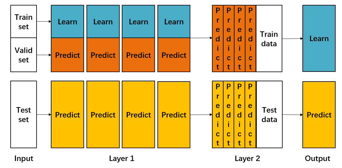
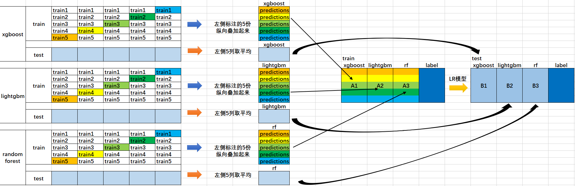
1. Divide the data set into training set and test_set, and conduct K-fold cross validation for the divided training set. For example, if the data set with 10000 samples is divided into 80% training and 20% testing for the first time, then test_ Set has 2000 samples and training data has 8000 samples. For the second time, divide the 8000 samples again and conduct 50% cross validation, then there will be five groups of 6400 training samples and 1600 training samples_ Set and valid_set.
2. Each cross validation is equivalent to training a model with 6400 blue data, verifying 1600 orange data with the model, and predicting the test set to obtain 2000 prediction results. In this way, after five cross tests, the results of 5 * 1600 verification sets in the middle orange (equivalent to the prediction results of each data) and the prediction results of 5 * 2000 test sets can be obtained.
3. Next, the 5 * 1600 prediction results of the verification set will be spliced into an 8000 long matrix, marked as 𝐵 1, and the prediction results of the 5 * 2000 row test set will be weighted average to obtain a matrix of 2000 rows and columns, marked as 𝐵 1.
4. The prediction results 𝐴 1 and 𝐵 1 of a base model on the data set are obtained above. In this way, when we integrate the three base models, we get six matrices: 𝐴 1, 𝐴 2, 𝐴 3, 𝐵 1, 𝐵 2 and 𝐵 3.
5. After that, we will combine 𝐴 1, 𝐴 2 and 𝐴 3 together into a matrix of 8000 rows and 3 columns as training data, and combine 𝐵 1, 𝐵 2 and 𝐵 3 together into a matrix of 2000 rows and 3 columns as testing data, so that the lower level learners can retrain based on such data.
6. Retraining is based on the prediction results of each basic model as features (three features). The secondary learner will learn how to give weight w to the prediction results of such basic learning to make the final prediction most accurate.

The schematic diagram of steps 1 and 2 is as above, and the schematic diagram of steps 3, 4, 5 and 6 is as follows.

Comparison between Stacking and Blending:

• The advantages of Blending are:
  Simpler than stacking (because there is no need to perform k times of cross validation to obtain the stacker feature)
• The disadvantages are:
  Very little data is used (hold out is divided as the test set, not cv)
  blender may be over fitted (in fact, the probability is caused by the first point)
  stacking CV S used multiple times will be more robust

2.2 code examples

## Import required libraries
from sklearn.model_selection import cross_val_score
from sklearn.linear_model import LogisticRegression
from sklearn.neighbors import KNeighborsClassifier
from sklearn.naive_bayes import GaussianNB 
from sklearn.ensemble import RandomForestClassifier
from mlxtend.classifier import StackingCVClassifier
from matplotlib import pyplot as plt

## Import iris dataset
from sklearn import datasets

iris = datasets.load_iris()
X, y = iris.data[:, 1:3], iris.target

## The basic models are constructed, which are KNN, RF and Bayesian classifiers respectively, and the second layer model is LR
RANDOM_SEED = 42

clf1 = KNeighborsClassifier(n_neighbors=1)
clf2 = RandomForestClassifier(random_state=RANDOM_SEED)
clf3 = GaussianNB()
lr = LogisticRegression()

# Starting from v0.18.0, StackingCVRegressor supports
# `random_state` to get deterministic result.
sclf = StackingCVClassifier(classifiers=[clf1, clf2, clf3],  # First layer classifier
                            meta_classifier=lr,   # Second layer classifier
                            random_state=RANDOM_SEED)

## Conduct 50% cross validation
print('5-fold cross validation:\n')

for clf, label in zip([clf1, clf2, clf3, sclf], ['KNN', 'Random Forest', 'Naive Bayes','StackingClassifier']):
    scores = cross_val_score(clf, X, y, cv=5, scoring='accuracy')
    print("Accuracy: %0.2f (+/- %0.2f) [%s]" % (scores.mean(), scores.std(), label))

5-fold cross validation:
Accuracy: 0.91 (+/- 0.07) [KNN]
Accuracy: 0.94 (+/- 0.04) [Random Forest]
Accuracy: 0.91 (+/- 0.04) [Naive Bayes]
Accuracy: 0.94 (+/- 0.04) [StackingClassifier]

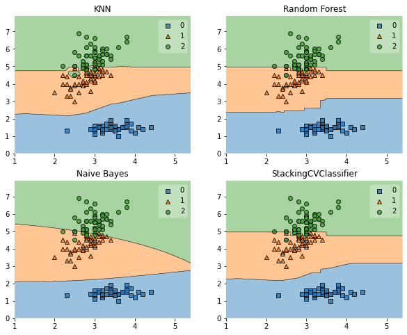
# We draw decision boundaries
from mlxtend.plotting import plot_decision_regions
import matplotlib.gridspec as gridspec
import itertools

gs = gridspec.GridSpec(2, 2)
fig = plt.figure(figsize=(10,8))
for clf, lab, grd in zip([clf1, clf2, clf3, sclf], 
                         ['KNN', 
                          'Random Forest', 
                          'Naive Bayes',
                          'StackingCVClassifier'],
                          itertools.product([0, 1], repeat=2)):
    clf.fit(X, y)
    ax = plt.subplot(gs[grd[0], grd[1]])
    fig = plot_decision_regions(X=X, y=y, clf=clf)
    plt.title(lab)
plt.show()

reference resources:
DataWhale open source content