Datawhale zero foundation entry data mining - Task3 Feature Engineering
3, Characteristic engineering objectives
Game Title: Zero basic entry data mining - used car transaction price prediction
3.1 characteristic engineering objectives
-
Further analyze the characteristics and process the data
-
Complete the analysis of characteristic engineering
3.2 content introduction
Common engineering features include:
- Exception handling:
- Delete outliers through box diagram (or 3-Sigma) analysis;
- BOX-COX conversion (processing biased distribution);
- Long tail truncation;
- Feature normalization / standardization:
- Standardization (conversion to standard normal distribution);
- Normalization (grasping and changing to [0,1] interval);
- For power-law distribution, the formula can be used: l o g ( 1 + x 1 + m e d i a n ) log(\frac{1+x}{1+median}) log(1+median1+x)
- Data bucket:
- Equal frequency bucket;
- Equidistant barrel separation;
- Best KS bucket classification (similar to secondary classification using Gini index);
- Chi square barrel separation;
- Missing value handling:
- No processing (for tree models such as XGBoost);
- Delete (too much missing data);
- Interpolation completion, including mean / median / mode / modeling prediction / multiple interpolation / compressed sensing completion / matrix completion, etc;
- Sub box, one box missing value;
- Characteristic structure:
- Construct statistical features and report counting, summation, proportion, standard deviation, etc;
- Time characteristics, including relative time and absolute time, holidays, weekends, etc;
- Geographic information, including box division, distribution coding and other methods;
- Nonlinear transformation, including log / square / root sign, etc;
- Feature combination, feature intersection;
- Benevolent people see benevolence, wise people see wisdom.
- Feature screening
- filter: first select the characteristics of the data, and then train the learner. The common methods are Relief / variance selection / correlation coefficient method / chi square test / mutual information method;
- Wrapper: directly take the performance of the learner to be used as the evaluation criterion of the feature subset. The common methods are LVM (Las Vegas Wrapper);
- embedding: combining filtering and wrapping, feature selection is automatically carried out in the process of learner training. lasso regression is common;
- Dimensionality reduction
- PCA/ LDA/ ICA;
- Feature selection is also a dimension reduction.
3.3 code example
3.3.0 importing data
# Import the libraries you need to use
import os
import pandas as pd
import numpy as np
from sklearn.preprocessing import LabelEncoder
from sklearn.preprocessing import MinMaxScaler
import lightgbm as lgb
from catboost import CatBoostRegressor
from sklearn.model_selection import KFold, RepeatedKFold
from sklearn.metrics import mean_absolute_error
from sklearn import linear_model
import warnings

warnings.filterwarnings('ignore')
Test_data = reduce_mem_usage(pd.read_csv('data/car_testA_0110.csv', sep=' '))
Train_data = reduce_mem_usage(pd.read_csv('data/car_train_0110.csv', sep=' '))
Train_data.shape
In fact, in the last section, we already have a basic idea of feature engineering. We won't repeat the basic information of data here.
3.3.1 delete outliers
3.3.1.1 data cleaning
Note: not all data here are used in this method. The process here is called data cleaning, but after practice, it will be found that 185138 pieces of data will be left after cleaning the data of this competition, and 1 \ 4 of the data will be deleted. Personally, I think it will destroy the comprehensiveness of the original data, so I didn't deal with it here.
# Here I wrap an exception handling code, which can be called at will.
def outliers_proc(data, col_name, scale=3):
    """
    Used to clean outliers. It is used by default box_plot(scale=3)Cleaning
    :param data: receive pandas data format
    :param col_name: pandas Listing
    :param scale: scale
    :return:
    """

    def box_plot_outliers(data_ser, box_scale):
        """
        Remove outliers using box diagram
        :param data_ser: receive pandas.Series data format
        :param box_scale: Dimension of box diagram,
        :return:
        """
        iqr = box_scale * (data_ser.quantile(0.75) - data_ser.quantile(0.25))
        val_low = data_ser.quantile(0.25) - iqr
        val_up = data_ser.quantile(0.75) + iqr
        rule_low = (data_ser < val_low)
        rule_up = (data_ser > val_up)
        return (rule_low, rule_up), (val_low, val_up)

    data_n = data.copy()
    data_series = data_n[col_name]
    rule, value = box_plot_outliers(data_series, box_scale=scale)
    index = np.arange(data_series.shape[0])[rule[0] | rule[1]]
    print("Delete number is: {}".format(len(index)))
    data_n = data_n.drop(index)
    data_n.reset_index(drop=True, inplace=True)
    print("Now column number is: {}".format(data_n.shape[0]))
    index_low = np.arange(data_series.shape[0])[rule[0]]
    outliers = data_series.iloc[index_low]
    print("Description of data less than the lower bound is:")
    print(pd.Series(outliers).describe())
    index_up = np.arange(data_series.shape[0])[rule[1]]
    outliers = data_series.iloc[index_up]
    print("Description of data larger than the upper bound is:")
    print(pd.Series(outliers).describe())

    fig, ax = plt.subplots(1, 2, figsize=(10, 7))
    sns.boxplot(y=data[col_name], data=data, palette="Set1", ax=ax[0])
    sns.boxplot(y=data_n[col_name], data=data_n, palette="Set1", ax=ax[1])
    return data_n
import matplotlib.pyplot as plt
import seaborn as sns
# Data cleaning
for i in [ 'v_8',  'v_23']:
    print(i)
    Train_data=outliers_proc(Train_data, i, scale=3)
v_8
Delete number is: 48536
Now column number is: 201464
Description of data less than the lower bound is:
count    4.853600e+04
mean     6.556511e-07
std      0.000000e+00
min      0.000000e+00
25%      0.000000e+00
50%      0.000000e+00
75%      0.000000e+00
max      6.532669e-04
Name: v_8, dtype: float64
Description of data larger than the upper bound is:
count    0.0
mean     NaN
std      NaN
min      NaN
25%      NaN
50%      NaN
75%      NaN
max      NaN
Name: v_8, dtype: float64
v_23
Delete number is: 16326
Now column number is: 185138
Description of data less than the lower bound is:
count    0.0
mean     NaN
std      NaN
min      NaN
25%      NaN
50%      NaN
75%      NaN
max      NaN
Name: v_23, dtype: float64
Description of data larger than the upper bound is:
count    1.632600e+04
mean              inf
std      5.332031e-01
min      4.511719e+00
25%      4.730469e+00
50%      4.988281e+00
75%      5.351562e+00
max      8.578125e+00
Name: v_23, dtype: float64
3.3.1.2 handling of other data outliers
Note: we found v when analyzing the data in the previous section_ 14 and price have some extreme values. Here, the extreme values are deleted as outliers.
Train_data = Train_data.drop(Train_data[Train_data['v_14']>8].index)
Train_data = Train_data.drop(Train_data[Train_data['price'] < 3].index)
3.3.1.3 reduce data memory occupation
def reduce_mem_usage(df):
    """ iterate through all the columns of a dataframe and modify the data type
        to reduce memory usage.
    """
    start_mem = df.memory_usage().sum()
    print('Memory usage of dataframe is {:.2f} MB'.format(start_mem))

    for col in df.columns:
        col_type = df[col].dtype

        if col_type != object:
            c_min = df[col].min()
            c_max = df[col].max()
            if str(col_type)[:3] == 'int':
                if c_min > np.iinfo(np.int8).min and c_max < np.iinfo(np.int8).max:
                    df[col] = df[col].astype(np.int8)
                elif c_min > np.iinfo(np.int16).min and c_max < np.iinfo(np.int16).max:
                    df[col] = df[col].astype(np.int16)
                elif c_min > np.iinfo(np.int32).min and c_max < np.iinfo(np.int32).max:
                    df[col] = df[col].astype(np.int32)
                elif c_min > np.iinfo(np.int64).min and c_max < np.iinfo(np.int64).max:
                    df[col] = df[col].astype(np.int64)
            else:
                if c_min > np.finfo(np.float16).min and c_max < np.finfo(np.float16).max:
                    df[col] = df[col].astype(np.float16)
                elif c_min > np.finfo(np.float32).min and c_max < np.finfo(np.float32).max:
                    df[col] = df[col].astype(np.float32)
                else:
                    df[col] = df[col].astype(np.float64)
        else:
            df[col] = df[col].astype('category')

    end_mem = df.memory_usage().sum()
    print('Memory usage after optimization is: {:.2f} MB'.format(end_mem))
    print('Decreased by {:.1f}%'.format(100 * (start_mem - end_mem) / start_mem))
    return df
3.3.2 characteristic structure
# The training set and test set are put together to facilitate the construction of features
Train_data['price'] = np.log1p(Train_data['price'])

# Merging facilitates subsequent operations
df = pd.concat([Train_data, Test_data], ignore_index=True)
# One hot coding is used for features with few categories
one_hot_list = ['fuelType','gearbox','notRepairedDamage','bodyType']
for col in one_hot_list:
    one_hot = pd.get_dummies(df[col])
    one_hot.columns = [col+'_'+str(i) for i in range(len(one_hot.columns))]
    df = pd.concat([df,one_hot],axis=1)
-
One hot coding is more accurate for data classification, and many machine learning algorithms can not be directly used for data classification. The category of data must be converted into numbers, and the input and output variables of classification are the same.
-
We can directly use integer coding and readjust it when necessary. This may apply to problems where there is a natural relationship between categories, such as labels with temperatures "cold" (0) and "hot" (1).
-
When there is no relationship, problems may arise. An example may be the labels "dog" and "cat". In these cases, we want to make the network more expressive and provide probabilistic numbers for each possible tag value. This is helpful for problem network modeling. When the output variable is encoded with one hot, it can provide a more accurate set of predictions than a single label.
Introduction to one hot coding:[ What is one hot coding? Why use one hot encoding- Zhihu (zhihu.com)](https://zhuanlan.zhihu.com/p/37471802)
## 1. The first step is to deal with useless values and basically unchanged values
#SaleID is definitely useless, but we can use it to count the number of group s with other features
#Name usually has nothing to dig, but there seem to be many with the same name. You can dig it
df['name_count'] = df.groupby(['name'])['SaleID'].transform('count')
# del df['name']

#seller has a special value. The training set is unique to the test set. Delete it
df.drop(df[df['seller'] == 0].index, inplace=True)
del df['offerType']
del df['seller']

## 2. The second step is to deal with the missing value
# Fill 0 with all of the following features
df['fuelType'] = df['fuelType'].fillna(0)
df['bodyType'] = df['bodyType'].fillna(0)
df['gearbox']=df['gearbox'].fillna(0)
df['notRepairedDamage']=df['notRepairedDamage'].fillna(0)
df['model'] = df['model'].fillna(0)

# 3. Step 3 exception value handling
# At present, according to the preliminary judgment of abnormal value, only the value of notrepaired damage is problematic, and there is power within the scope specified in the title. Deal with it
df['power'] = df['power'].map(lambda x: 600 if x>600 else x)
df['notRepairedDamage'] = df['notRepairedDamage'].astype('str').apply(lambda x: x if x != '-' else None).astype('float32')
Note: here is the whole process of my feature engineering. Welcome to discuss with the big guys.
## 1. Time, area or something
#time
from datetime import datetime
def date_process(x):
    year = int(str(x)[:4])
    month = int(str(x)[4:6])
    day = int(str(x)[6:8])

    if month < 1:
        month = 1

    date = datetime(year, month, day)
    return date

df['regDate'] = df['regDate'].apply(date_process)
df['creatDate'] = df['creatDate'].apply(date_process)
df['regDate_year'] = df['regDate'].dt.year
df['regDate_month'] = df['regDate'].dt.month
df['regDate_day'] = df['regDate'].dt.day
df['creatDate_year'] = df['creatDate'].dt.year
df['creatDate_month'] = df['creatDate'].dt.month
df['creatDate_day'] = df['creatDate'].dt.day
df['car_age_day'] = (df['creatDate'] - df['regDate']).dt.days
df['car_age_year'] = round(df['car_age_day'] / 365, 1)

df['year_kilometer'] = df['kilometer'] / df['car_age_year']

#region
df['regionCode_count'] = df.groupby(['regionCode'])['SaleID'].transform('count')
df['city'] = df['regionCode'].apply(lambda x : str(x)[:2])


## 2. Classification features
# Classify the continuous features that can be classified into buckets. The kilometer has been divided into buckets
bin = [i*10 for i in range(31)]
df['power_bin'] = pd.cut(df['power'], bin, labels=False)
tong = df[['power_bin', 'power']].head()


bin = [i*10 for i in range(24)]
df['model_bin'] = pd.cut(df['model'], bin, labels=False)
tong = df[['model_bin', 'model']].head()

# The classification features with a little more value are combined with price, and many groups are made. However, in the final use, each group is tested separately to select the features of real work
Train_gb = Train_data.groupby("regionCode")
all_info = {}
for kind, kind_data in Train_gb:
    info = {}
    kind_data = kind_data[kind_data['price'] > 0]
    info['regionCode_amount'] = len(kind_data)
    info['regionCode_price_max'] = kind_data.price.max()
    info['regionCode_price_median'] = kind_data.price.median()
    info['regionCode_price_min'] = kind_data.price.min()
    info['regionCode_price_sum'] = kind_data.price.sum()
    info['regionCode_price_std'] = kind_data.price.std()
    info['regionCode_price_mean'] = kind_data.price.mean()
    info['regionCode_price_skew'] = kind_data.price.skew()
    info['regionCode_price_kurt'] = kind_data.price.kurt()
    info['regionCode_mad'] = kind_data.price.mad()

    all_info[kind] = info
brand_fe = pd.DataFrame(all_info).T.reset_index().rename(columns={"index": "regionCode"})
df = df.merge(brand_fe, how='left', on='regionCode')

Train_gb = Train_data.groupby("brand")
all_info = {}
for kind, kind_data in Train_gb:
    info = {}
    kind_data = kind_data[kind_data['price'] > 0]
    info['brand_amount'] = len(kind_data)
    info['brand_price_max'] = kind_data.price.max()
    info['brand_price_median'] = kind_data.price.median()
    info['brand_price_min'] = kind_data.price.min()
    info['brand_price_sum'] = kind_data.price.sum()
    info['brand_price_std'] = kind_data.price.std()
    info['brand_price_mean'] = kind_data.price.mean()
    info['brand_price_skew'] = kind_data.price.skew()
    info['brand_price_kurt'] = kind_data.price.kurt()
    info['brand_price_mad'] = kind_data.price.mad()

    all_info[kind] = info
brand_fe = pd.DataFrame(all_info).T.reset_index().rename(columns={"index": "brand"})
df = df.merge(brand_fe, how='left', on='brand')

Train_gb = df.groupby("model_bin")
all_info = {}
for kind, kind_data in Train_gb:
    info = {}
    kind_data = kind_data[kind_data['price'] > 0]
    info['model_amount'] = len(kind_data)
    info['model_price_max'] = kind_data.price.max()
    info['model_price_median'] = kind_data.price.median()
    info['model_price_min'] = kind_data.price.min()
    info['model_price_sum'] = kind_data.price.sum()
    info['model_price_std'] = kind_data.price.std()
    info['model_price_mean'] = kind_data.price.mean()
    info['model_price_skew'] = kind_data.price.skew()
    info['model_price_kurt'] = kind_data.price.kurt()
    info['model_price_mad'] = kind_data.price.mad()
    all_info[kind] = info
brand_fe = pd.DataFrame(all_info).T.reset_index().rename(columns={"index": "model"})
df = df.merge(brand_fe, how='left', on='model')

Train_gb = Train_data.groupby("kilometer")
all_info = {}
for kind, kind_data in Train_gb:
    info = {}
    kind_data = kind_data[kind_data['price'] > 0]
    info['kilometer_amount'] = len(kind_data)
    info['kilometer_price_max'] = kind_data.price.max()
    info['kilometer_price_median'] = kind_data.price.median()
    info['kilometer_price_min'] = kind_data.price.min()
    info['kilometer_price_sum'] = kind_data.price.sum()
    info['kilometer_price_std'] = kind_data.price.std()
    info['kilometer_price_mean'] = kind_data.price.mean()
    info['kilometer_price_skew'] = kind_data.price.skew()
    info['kilometer_price_kurt'] = kind_data.price.kurt()
    info['kilometer_price_mad'] = kind_data.price.mad()

    all_info[kind] = info
brand_fe = pd.DataFrame(all_info).T.reset_index().rename(columns={"index": "kilometer"})
df = df.merge(brand_fe, how='left', on='kilometer')

Train_gb = Train_data.groupby("bodyType")
all_info = {}
for kind, kind_data in Train_gb:
    info = {}
    kind_data = kind_data[kind_data['price'] > 0]
    info['bodyType_amount'] = len(kind_data)
    info['bodyType_price_max'] = kind_data.price.max()
    info['bodyType_price_median'] = kind_data.price.median()
    info['bodyType_price_min'] = kind_data.price.min()
    info['bodyType_price_sum'] = kind_data.price.sum()
    info['bodyType_price_std'] = kind_data.price.std()
    info['bodyType_price_mean'] = kind_data.price.mean()
    info['bodyType_price_skew'] = kind_data.price.skew()
    info['bodyType_price_kurt'] = kind_data.price.kurt()
    info['bodyType_price_mad'] = kind_data.price.mad()

    all_info[kind] = info
brand_fe = pd.DataFrame(all_info).T.reset_index().rename(columns={"index": "bodyType"})
df = df.merge(brand_fe, how='left', on='bodyType')


Train_gb = Train_data.groupby("fuelType")
all_info = {}
for kind, kind_data in Train_gb:
    info = {}
    kind_data = kind_data[kind_data['price'] > 0]
    info['fuelType_amount'] = len(kind_data)
    info['fuelType_price_max'] = kind_data.price.max()
    info['fuelType_price_median'] = kind_data.price.median()
    info['fuelType_price_min'] = kind_data.price.min()
    info['fuelType_price_sum'] = kind_data.price.sum()
    info['fuelType_price_std'] = kind_data.price.std()
    info['fuelType_price_mean'] = kind_data.price.mean()
    info['fuelType_price_skew'] = kind_data.price.skew()
    info['fuelType_price_kurt'] = kind_data.price.kurt()
    info['fuelType_price_mad'] = kind_data.price.mad()

    all_info[kind] = info
brand_fe = pd.DataFrame(all_info).T.reset_index().rename(columns={"index": "fuelType"})
df = df.merge(brand_fe, how='left', on='fuelType')


Train_gb = Train_data.groupby("v_8")
all_info = {}
for kind, kind_data in Train_gb:
    info = {}
    kind_data = kind_data[kind_data['price'] > 0]
    info['v_8_amount'] = len(kind_data)
    info['v_8_price_max'] = kind_data.price.max()
    info['v_8_price_median'] = kind_data.price.median()
    info['v_8_price_min'] = kind_data.price.min()
    info['v_8_price_sum'] = kind_data.price.sum()
    info['v_8_price_std'] = kind_data.price.std()
    info['v_8_price_mean'] = kind_data.price.mean()
    info['v_8_price_skew'] = kind_data.price.skew()
    info['v_8_price_kurt'] = kind_data.price.kurt()
    info['v_8_price_mad'] = kind_data.price.mad()

    all_info[kind] = info
brand_fe = pd.DataFrame(all_info).T.reset_index().rename(columns={"index": "v_8"})
df = df.merge(brand_fe, how='left', on='v_8')


Train_gb = df.groupby('car_age_year')
all_info = {}
for kind, kind_data in Train_gb:
    info = {}
    kind_data = kind_data[kind_data['price'] > 0]
    info['car_age_year_amount'] = len(kind_data)
    info['car_age_year_price_max'] = kind_data.price.max()
    info['car_age_year_price_median'] = kind_data.price.median()
    info['car_age_year_price_min'] = kind_data.price.min()
    info['car_age_year_price_sum'] = kind_data.price.sum()
    info['car_age_year_price_std'] = kind_data.price.std()
    info['car_age_year_price_mean'] = kind_data.price.mean()
    info['car_age_year_price_skew'] = kind_data.price.skew()
    info['car_age_year_price_kurt'] = kind_data.price.kurt()
    info['car_age_year_price_mad'] = kind_data.price.mad()

    all_info[kind] = info
brand_fe = pd.DataFrame(all_info).T.reset_index().rename(columns={"index": "car_age_year"})
df = df.merge(brand_fe, how='left', on='car_age_year')


# When testing the classification features and price, it is found that there is some effect, and the model is processed immediately
for kk in [ "regionCode","brand","model","bodyType","fuelType"]:
    Train_gb = df.groupby(kk)
    all_info = {}
    for kind, kind_data in Train_gb:
        info = {}
        kind_data = kind_data[kind_data['car_age_day'] > 0]
        info[kk+'_days_max'] = kind_data.car_age_day.max()
        info[kk+'_days_min'] = kind_data.car_age_day.min()
        info[kk+'_days_std'] = kind_data.car_age_day.std()
        info[kk+'_days_mean'] = kind_data.car_age_day.mean()
        info[kk+'_days_median'] = kind_data.car_age_day.median()
        info[kk+'_days_sum'] = kind_data.car_age_day.sum()
        all_info[kind] = info
    brand_fe = pd.DataFrame(all_info).T.reset_index().rename(columns={"index": kk})
    df = df.merge(brand_fe, how='left', on=kk)

    Train_gb = df.groupby(kk)
    all_info = {}
    for kind, kind_data in Train_gb:
        info = {}
        kind_data = kind_data[kind_data['power'] > 0]
        info[kk+'_power_max'] = kind_data.power.max()
        info[kk+'_power_min'] = kind_data.power.min()
        info[kk+'_power_std'] = kind_data.power.std()
        info[kk+'_power_mean'] = kind_data.power.mean()
        info[kk+'_power_median'] = kind_data.power.median()
        info[kk+'_power_sum'] = kind_data.power.sum()
        all_info[kind] = info
    brand_fe = pd.DataFrame(all_info).T.reset_index().rename(columns={"index": kk})
    df = df.merge(brand_fe, how='left', on=kk)

    Train_gb = df.groupby(kk)
    all_info = {}
    for kind, kind_data in Train_gb:
        info = {}
        kind_data = kind_data[kind_data['v_0'] > 0]
        info[kk+'_v_0_max'] = kind_data.v_0.max()
        info[kk+'_v_0_min'] = kind_data.v_0.min()
        info[kk+'_v_0_std'] = kind_data.v_0.std()
        info[kk+'_v_0_mean'] = kind_data.v_0.mean()
        info[kk+'_v_0_median'] = kind_data.v_0.median()
        info[kk+'_v_0_sum'] = kind_data.v_0.sum()
        all_info[kind] = info
    brand_fe = pd.DataFrame(all_info).T.reset_index().rename(columns={"index": kk})
    df = df.merge(brand_fe, how='left', on=kk)

    Train_gb = df.groupby(kk)
    all_info = {}
    for kind, kind_data in Train_gb:
        info = {}
        kind_data = kind_data[kind_data['v_3'] > 0]
        info[kk+'_v_3_max'] = kind_data.v_3.max()
        info[kk+'_v_3_min'] = kind_data.v_3.min()
        info[kk+'_v_3_std'] = kind_data.v_3.std()
        info[kk+'_v_3_mean'] = kind_data.v_3.mean()
        info[kk+'_v_3_median'] = kind_data.v_3.median()
        info[kk+'_v_3_sum'] = kind_data.v_3.sum()
        all_info[kind] = info
    brand_fe = pd.DataFrame(all_info).T.reset_index().rename(columns={"index": kk})
    df = df.merge(brand_fe, how='left', on=kk)

    Train_gb = df.groupby(kk)
    all_info = {}
    for kind, kind_data in Train_gb:
        info = {}
        kind_data = kind_data[kind_data['v_16'] > 0]
        info[kk+'_v_16_max'] = kind_data.v_16.max()
        info[kk+'_v_16_min'] = kind_data.v_16.min()
        info[kk+'_v_16_std'] = kind_data.v_16.std()
        info[kk+'_v_16_mean'] = kind_data.v_16.mean()
        info[kk+'_v_16_median'] = kind_data.v_16.median()
        info[kk+'_v_16_sum'] = kind_data.v_16.sum()
        all_info[kind] = info
    brand_fe = pd.DataFrame(all_info).T.reset_index().rename(columns={"index": kk})
    df = df.merge(brand_fe, how='left', on=kk)

    Train_gb = df.groupby(kk)
    all_info = {}
    for kind, kind_data in Train_gb:
        info = {}
        kind_data = kind_data[kind_data['v_18'] > 0]
        info[kk+'_v_18_max'] = kind_data.v_16.max()
        info[kk+'_v_18_min'] = kind_data.v_16.min()
        info[kk+'_v_18_std'] = kind_data.v_16.std()
        info[kk+'_v_18_mean'] = kind_data.v_16.mean()
        info[kk+'_v_18_median'] = kind_data.v_16.median()
        info[kk+'_v_18_sum'] = kind_data.v_16.sum()
        all_info[kind] = info
    brand_fe = pd.DataFrame(all_info).T.reset_index().rename(columns={"index": kk})
    df = df.merge(brand_fe, how='left', on=kk)

## 3. Continuous numerical characteristics
# They are all anonymous features. After comparing the distribution of training sets and test sets, there is basically no problem. Let's keep them all for the time being
# In the later stage, we may have to eliminate those with high similarity
# The price is characterized by several continuous numerical features with high feature importance output from the simple lgb model
# kk="regionCode"
# # dd = 'v_3'[0, 3, 6, 11, 16, 17, 18]
# for dd in ['v_0','v_1','v_3','v_16','v_17','v_18','v_22','v_23']:
#     Train_gb = df.groupby(kk)
#     all_info = {}
#     for kind, kind_data in Train_gb:
#         info = {}
#         kind_data = kind_data[kind_data[dd] > -10000000]
#         info[kk+'_'+dd+'_max'] = kind_data[dd].max()
#         info[kk+'_'+dd+'_min'] = kind_data[dd].min()
#         info[kk+'_'+dd+'_std'] = kind_data[dd].std()
#         info[kk+'_'+dd+'_mean'] = kind_data[dd].mean()
#         info[kk+'_'+dd+'_median'] = kind_data[dd].median()
#         info[kk+'_'+dd+'_sum'] = kind_data[dd].sum()
#         all_info[kind] = info
#     brand_fe = pd.DataFrame(all_info).T.reset_index().rename(columns={"index": kk})
#     df = df.merge(brand_fe, how='left', on=kk)


# dd = 'v_0'
# Train_gb = df.groupby(kk)
# all_info = {}
# for kind, kind_data in Train_gb:
#     info = {}
#     kind_data = kind_data[kind_data[dd]> -10000000]
#     info[kk+'_'+dd+'_max'] = kind_data.v_0.max()
#     info[kk+'_'+dd+'_min'] = kind_data.v_0.min()
#     info[kk+'_'+dd+'_std'] = kind_data.v_0.std()
#     info[kk+'_'+dd+'_mean'] = kind_data.v_0.mean()
#     info[kk+'_'+dd+'_median'] = kind_data.v_0.median()
#     info[kk+'_'+dd+'_sum'] = kind_data.v_0.sum()
#     all_info[kind] = info
#     all_info[kind] = info
# brand_fe = pd.DataFrame(all_info).T.reset_index().rename(columns={"index": kk})
# df = df.merge(brand_fe, how='left', on=kk)
for i in ['v_0', 'v_1', 'v_2', 'v_3', 'v_4', 'v_5', 'v_6', 'v_7', 'v_8', 'v_9', 'v_10','v_11', 'v_12', 'v_13', 'v_14', 'v_15', 'v_16', 'v_17', 'v_18', 'v_19', 'v_20', 'v_21', 'v_22','v_23']:
    df[i+'**2']=df[i]**2
    df[i+'**3']=df[i]**3
    df[i+'log']=np.log1p(df[i])
## Constructing polynomial features


df['v_0_2']=(df['v_0'])**2

df['v_3_6']=(df['v_3'])**6
df['v_3_9']=(df['v_3'])**9

df['v_6_8']=(df['v_6'])**8

df['v_7_2']=(df['v_7'])**2
df['v_7_8']=(df['v_7'])**8
df['v_7_12']=(df['v_7'])**12

df['v_10_6']=(df['v_10'])**6

df['v_11_2']=(df['v_11'])**2
df['v_11_3']=(df['v_11'])**3
df['v_11_4']=(df['v_11'])**4
df['v_11_6']=(df['v_11'])**6
df['v_11_8']=(df['v_11'])**8
df['v_11_9']=(df['v_11'])**9

for i in [2,3,4,6,8]:
    df['v_15_'+str(i)]=(df['v_15'])**i

df['v_16_6']=(df['v_16'])**6

df['v_18_9']=(df['v_18'])**9

df['v_21_8']=(df['v_21'])**8

df['v_22_2']=(df['v_22'])**2
df['v_22_8']=(df['v_22'])**8
df['v_22_12']=(df['v_22'])**12

df['v_23_9']=(df['v_23'])**9
df['v_23_18']=(df['v_23'])**18
for i in [2,3,4,27,18]:
    df['kilometer_'+str(i)]=(df['kilometer'])**i
for i in [8,9,27,18]:
    df['bodyType_'+str(i)]=(df['bodyType'])**i
for i in [2,3,4,6,8,9,12,28]:
    df['gearbox_'+str(i)]=(df['gearbox'])**i
## It mainly carries out feature cross between anonymous features and several classification features with high importance
#The first batch of characteristic projects
for i in range(24):#range(23)
    for j in range(24):
        df['new'+str(i)+'*'+str(j)]=df['v_'+str(i)]*df['v_'+str(j)]


#The second batch of characteristic projects
for i in range(24):
    for j in range(24):
        df['new'+str(i)+'+'+str(j)]=df['v_'+str(i)]+df['v_'+str(j)]

# # The third batch of characteristic projects
for i in range(24):
    df['new' + str(i) + '*power'] = df['v_' + str(i)] * df['power']

for i in range(24):
    df['new' + str(i) + '*day'] = df['v_' + str(i)] * df['car_age_day']

for i in range(24):
    df['new' + str(i) + '*year'] = df['v_' + str(i)] * df['car_age_year']


# #The fourth batch of characteristic projects
for i in range(24):
    for j in range(24):
        df['new'+str(i)+'-'+str(j)]=df['v_'+str(i)]-df['v_'+str(j)]
        df['new'+str(i)+'/'+str(j)]=df['v_'+str(i)]/df['v_'+str(j)]
'''
Polynomial features, tested to be the best of order 3
'''
from sklearn import preprocessing
feature_cols = [ 'v_0', 'v_3','v_18', 'v_16']
poly_data = df[feature_cols]
poly = preprocessing.PolynomialFeatures(3,interaction_only=True)
poly_data_ndarray = poly.fit_transform(poly_data)
poly_data_final = pd.DataFrame(poly_data_ndarray,columns=poly.get_feature_names(poly_data.columns))
poly_data_final.drop(columns=[  'v_0', 'v_3','v_18', 'v_16'],inplace=True)
# Splice the secondary converted data to the original data set
df =pd.merge(df,poly_data_final, how='left',right_index=True,left_index=True)
df.drop(columns=['1'],inplace=True)

# Replace inf class data
df.replace([np.inf,-np.inf],np.nan,inplace=True)
# df=df.fillna(method='ffill')
feature_aggs = {}
# for i in sparse_feature:
for i in ['name', 'model', 'regionCode']:
    feature_aggs[i] = ['count', 'nunique']
for j in ['power', 'kilometer', 'car_age_day']:#,'v_4','v_8','v_10','v_12','v_13'
    feature_aggs[j] = ['mean','max','min','std','median','count']
def create_new_feature(df):
    result = df.copy()
#     for feature in sparse_feature:
    for feature in ['name', 'model', 'regionCode']:
        aggs = feature_aggs.copy()
        aggs.pop(feature)
        grouped = result.groupby(feature).agg(aggs)
        grouped.columns = ['{}_{}_{}'.format(feature, i[0], i[1]) for i in grouped.columns]
        grouped = grouped.reset_index().rename(columns={0: feature})
        result = pd.merge(result, grouped, how='left', on=feature)
    return result
df = create_new_feature(df)
from tqdm import *
from scipy.stats import entropy

feat_cols = []

### count code
for f in tqdm(['car_age_year','model', 'brand', 'regionCode']):
    df[f + '_count'] = df[f].map(df[f].value_counts())
    feat_cols.append(f + '_count')

# ### The category features are statistically characterized by numerical features, and several anonymous features with the highest correlation with price are randomly selected
# for f1 in tqdm(['model', 'brand', 'regionCode']):
#     group = data.groupby(f1, as_index=False)
#     for f2 in tqdm(['v_0', 'v_3', 'v_8', 'v_12']):
#         feat = group[f2].agg({
#             '{}_{}_max'.format(f1, f2): 'max', '{}_{}_min'.format(f1, f2): 'min',
#             '{}_{}_median'.format(f1, f2): 'median', '{}_{}_mean'.format(f1, f2): 'mean',
#             '{}_{}_std'.format(f1, f2): 'std', '{}_{}_mad'.format(f1, f2): 'mad'
#         })
#         data = data.merge(feat, on=f1, how='left')
#         feat_list = list(feat)
#         feat_list.remove(f1)
#         feat_cols.extend(feat_list)


### Second order intersection of category features
for f_pair in tqdm([['model', 'brand'], ['model', 'regionCode'], ['brand', 'regionCode']]):
    ### Co occurrence times
    df['_'.join(f_pair) + '_count'] = df.groupby(f_pair)['SaleID'].transform('count')
    ### nunique, entropy
    df = df.merge(df.groupby(f_pair[0], as_index=False)[f_pair[1]].agg({
        '{}_{}_nunique'.format(f_pair[0], f_pair[1]): 'nunique',
        '{}_{}_ent'.format(f_pair[0], f_pair[1]): lambda x: entropy(x.value_counts() / x.shape[0])
    }), on=f_pair[0], how='left')
    df = df.merge(df.groupby(f_pair[1], as_index=False)[f_pair[0]].agg({
        '{}_{}_nunique'.format(f_pair[1], f_pair[0]): 'nunique',
        '{}_{}_ent'.format(f_pair[1], f_pair[0]): lambda x: entropy(x.value_counts() / x.shape[0])
    }), on=f_pair[1], how='left')
    ### Proportional preference
    df['{}_in_{}_prop'.format(f_pair[0], f_pair[1])] = df['_'.join(f_pair) + '_count'] / df[f_pair[1] + '_count']
    df['{}_in_{}_prop'.format(f_pair[1], f_pair[0])] = df['_'.join(f_pair) + '_count'] / df[f_pair[0] + '_count']

    feat_cols.extend([
        '_'.join(f_pair) + '_count',
        '{}_{}_nunique'.format(f_pair[0], f_pair[1]), '{}_{}_ent'.format(f_pair[0], f_pair[1]),
        '{}_{}_nunique'.format(f_pair[1], f_pair[0]), '{}_{}_ent'.format(f_pair[1], f_pair[0]),
        '{}_in_{}_prop'.format(f_pair[0], f_pair[1]), '{}_in_{}_prop'.format(f_pair[1], f_pair[0])
    ])
The above is the process of feature construction. For more than 1000 features, there will certainly be many features that have a negative effect on the prediction results, and there will also be some features with high correlation and feature honor. Let's do feature screening next.
3.3.3 feature screening
1) Filter type
# correlation analysis
f=[]
numerical_cols = df.select_dtypes(exclude='object').columns
feature_cols = [col for col in numerical_cols  if
             col  not in['name','regDate','creatDate','model','brand','regionCode','seller','regDates','creatDates']]
for i in feature_cols:
    print(i,df[i].corr(df['price'], method='spearman'))
    f.append([i,df[i].corr(df['price'], method='spearman')])
f.sort(key=lambda x:x[1])

f.sort(key=lambda x:abs(x[1]),reverse=True)
new_f=[]
for i ,j in f:
    if abs(j)>0.8:
        new_f.append(i)
    print(i,j)
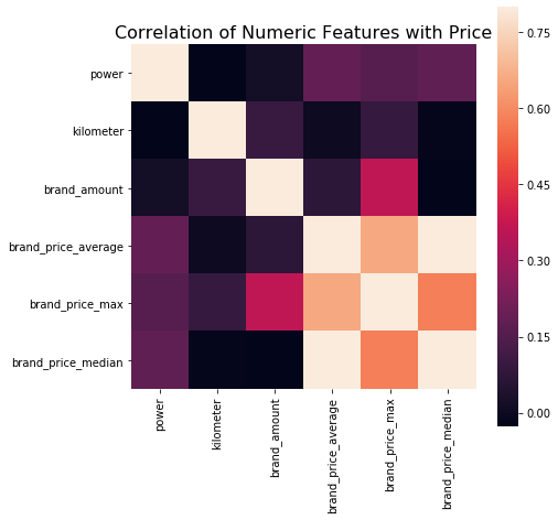
Here we only look at the features with a correlation of more than 0.8 with price. Other features have little significance for the prediction effect of price and are not considered.
# Of course, you can also look at the picture directly
data_numeric = data[['power', 'kilometer', 'brand_amount', 'brand_price_average',
                     'brand_price_max', 'brand_price_median']]
correlation = data_numeric.corr()

f , ax = plt.subplots(figsize = (7, 7))
plt.title('Correlation of Numeric Features with Price',y=1,size=16)
sns.heatmap(correlation,square = True,  vmax=0.8)
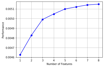
2) Wrapped
!pip install mlxtend
# k_ The feature is too big to run. There is no server, so interrupt in advance
from mlxtend.feature_selection import SequentialFeatureSelector as SFS
from sklearn.linear_model import LinearRegression
sfs = SFS(LinearRegression(),
           k_features=10,
           forward=True,
           floating=False,
           scoring = 'r2',
           cv = 0)
x = data.drop(['price'], axis=1)
x = x.fillna(0)
y = data['price']
sfs.fit(x, y)
sfs.k_feature_names_
The above code has been running for too long. It is not recommended to try.
# Draw it and you can see the marginal benefit
from mlxtend.plotting import plot_sequential_feature_selection as plot_sfs
import matplotlib.pyplot as plt
fig1 = plot_sfs(sfs.get_metric_dict(), kind='std_dev')
plt.grid()
plt.show()
3.4 experience summary
Feature engineering is the most important part of the competition. The quality of feature engineering often determines the final ranking and achievement.
It is part of the purpose of engineering data expression.
- Some competitions are characterized by anonymous features, which makes us not clear the direct correlation between features. At this time, we can only process based on features, such as packing, groupby and so on. In addition, we can further transform the features such as log and exp, Or perform four operations on multiple features (such as the service time calculated above), polynomial combination, etc., and then filter them. The anonymity of features actually limits the processing of features. Of course, sometimes using NN to extract some features will also achieve unexpected good results.
- For feature engineering that knows the meaning of features (non anonymous), especially in industrial type competitions, it will build more practical features based on signal processing, frequency domain extraction, abundance, skewness and so on. This is the feature construction combined with the background, which is also the case in the recommendation system, including various types of click through rate statistics, statistics of each period, statistics of user attributes and so on, Such a feature construction often needs to deeply analyze the business logic or physical principles behind it, so as to better find magic.
Of course, feature engineering is actually combined with the model, which is why it is necessary to divide buckets and normalize features for LR NN, and the processing effect and importance of features are often verified by the model.
Generally speaking, feature engineering is a simple entry, but it is very difficult to master it.