Datawhale zero foundation entry data mining Task5 model fusion

5, Model fusion

Game Title: Zero basic entry data mining - used car transaction price prediction

5.1 model fusion objectives

• Model fusion is carried out for the models completed by multiple parameters adjustment.
• Complete the fusion of multiple models.

5.2 content introduction

Model fusion is an important link in the later stage of the competition. Generally speaking, there are the following types and methods.

1. Simple weighted fusion:
   • Regression (classification probability): Arithmetic mean, Geometric mean;
   • Category: voting
   • Synthesis: rank averaging, log merging
2. stacking/blending:
   • Build a multi-layer model, and use the prediction results to fit the prediction.
3. In gbdt, boost:
   • Multi tree lifting method

5.3 introduction to stacking theory

1) What is stacking

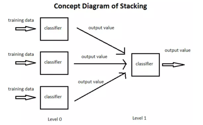
In short, stacking is to learn a new learner by taking the prediction results of these learners as a new training set after learning several basic learners with the initial training data.

The method used when combining individual learners is called combination strategy. For the classification problem, we can use the voting method to select the class with the most output. For the regression problem, we can average the results output by the classifier.

The above-mentioned voting method and average method are very effective combination strategies. Another combination strategy is to use another machine learning algorithm to combine the results of individual machine learners. This method is Stacking.

In the stacking method, we call the individual learner as the primary learner, the learner used for combination as the secondary learner or meta learner, and the data used for training by the secondary learner as the secondary training set. The secondary training set is obtained by using the primary learner on the training set.

2) How to stack

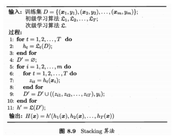
Quoted from watermelon book machine learning

• Process 1-3 is to train individual learners, that is, primary learners.
• Process 5-9 uses the trained individual learner to predict the result, and the predicted result is used as the training set of the secondary learner.
• Process 11 is to train the secondary learner with the predicted results of the primary learner and get the model we finally trained.

3) Explanation of Stacking method

First, let's start with a "not so correct" but easy to understand Stacking method.

Stacking model is essentially a hierarchical structure. For simplicity, only secondary stacking is analyzed here Suppose we have two base models, Model1_1,Model1_2 and a secondary model

Step 1. Base model Model1_1. Train the training set, and then use it to predict the label columns of train and test, which are P1 and T1 respectively

Model1_1. Model training:

KaTeX parse error: Expected '}', got '_' at position 118: ...^{\text {Model1_̲1 Train} }\left...

Model 1 after training_ 1 predict on train and test respectively, and the prediction labels are P1 and T1 respectively

KaTeX parse error: Expected '}', got '_' at position 118: ...^{\text {Model1_̲1 Predict} }\le...

KaTeX parse error: Expected '}', got '_' at position 117: ...^{\text {Model1_̲1 Predict} }\le...

Step 2. Base model Model1_2. Train the training set, and then use it to predict the label columns of train and test, which are P2 and T2 respectively

Model1_2 model training:

KaTeX parse error: Expected '}', got '_' at position 118: ...^{\text {Model1_̲2 Train} }\left...

Model 1 after training_ 2 predict on train and test respectively, and the prediction labels are P2 and T2 respectively

KaTeX parse error: Expected '}', got '_' at position 118: ...^{\text {Model1_̲2 Predict} }\le...

KaTeX parse error: Expected '}', got '_' at position 117: ...^{\text {Model1_̲2 Predict} }\le...

Step 3. P1,P2, T1 and T2 are combined to obtain a new training set and test set train2 and test2

KaTeX parse error: Expected '}', got '_' at position 155: ...}^{\text {Train_̲2 }} and \overb...

Then use the secondary model Model2 to train with the label of the real training set as the label, train with train2 as the feature, predict test2, and get the label column predicted by the final test set Y P r e Y_{Pre} YPre​.

KaTeX parse error: Expected '}', got '_' at position 155: ...}^{\text {Train_̲2 }} \overbrace...

KaTeX parse error: Expected '}', got '_' at position 154: ...)}^{\text {Test_̲2 }} \overbrace...

This is a basic original idea of our two-tier stacking. Based on the prediction results of different models, a layer of model is added for retraining, so as to obtain the final prediction of the model.

Stacking is essentially such a direct idea, but sometimes there is a problem when the distribution of the training set and the test set is not so consistent. The problem is that using the label trained by the initial model and then using the real label for retraining will undoubtedly lead to a certain model over fitting the training set, In this way, the generalization ability or effect of the model on the test set may be reduced to a certain extent. Therefore, the problem now becomes how to reduce the over fitting of retraining. Here we generally have two methods.

• 1. The simple linear model shall be selected for the secondary model as far as possible
• 1. Using K-fold cross validation

K-fold cross validation: training:

forecast:

5.4 code examples

5.4.1 regression \ classification probability fusion:

1) Simple weighted average, direct fusion of results

## Generate some simple sample data, test_prei represents the predicted value of the ith model
test_pre1 = [1.2, 3.2, 2.1, 6.2]
test_pre2 = [0.9, 3.1, 2.0, 5.9]
test_pre3 = [1.1, 2.9, 2.2, 6.0]

# y_test_true represents the true value of the second model
y_test_true = [1, 3, 2, 6] 
import numpy as np
import pandas as pd

## Define the weighted average function of the results
def Weighted_method(test_pre1,test_pre2,test_pre3,w=[1/3,1/3,1/3]):
    Weighted_result = w[0]*pd.Series(test_pre1)+w[1]*pd.Series(test_pre2)+w[2]*pd.Series(test_pre3)
    return Weighted_result
from sklearn import metrics
# MAE is calculated based on the prediction results of each model
print('Pred1 MAE:',metrics.mean_absolute_error(y_test_true, test_pre1))
print('Pred2 MAE:',metrics.mean_absolute_error(y_test_true, test_pre2))
print('Pred3 MAE:',metrics.mean_absolute_error(y_test_true, test_pre3))
Pred1 MAE: 0.175
Pred2 MAE: 0.075
Pred3 MAE: 0.1
## MAE is calculated according to weighting
w = [0.3,0.4,0.3] # Define specific gravity weight
Weighted_pre = Weighted_method(test_pre1,test_pre2,test_pre3,w)
print('Weighted_pre MAE:',metrics.mean_absolute_error(y_test_true, Weighted_pre))
Weighted_pre MAE: 0.0575

It can be found that the weighted results are improved compared with the previous results, which we call simple weighted average.

There are also some special forms, such as mean average and median average

## Define the weighted average function of the results
def Mean_method(test_pre1,test_pre2,test_pre3):
    Mean_result = pd.concat([pd.Series(test_pre1),pd.Series(test_pre2),pd.Series(test_pre3)],axis=1).mean(axis=1)
    return Mean_result
Mean_pre = Mean_method(test_pre1,test_pre2,test_pre3)
print('Mean_pre MAE:',metrics.mean_absolute_error(y_test_true, Mean_pre))
Mean_pre MAE: 0.0666666666667
## Define the weighted average function of the results
def Median_method(test_pre1,test_pre2,test_pre3):
    Median_result = pd.concat([pd.Series(test_pre1),pd.Series(test_pre2),pd.Series(test_pre3)],axis=1).median(axis=1)
    return Median_result
Median_pre = Median_method(test_pre1,test_pre2,test_pre3)
print('Median_pre MAE:',metrics.mean_absolute_error(y_test_true, Median_pre))
Median_pre MAE: 0.075

2) Stacking fusion (regression):

from sklearn import linear_model

def Stacking_method(train_reg1,train_reg2,train_reg3,y_train_true,test_pre1,test_pre2,test_pre3,model_L2= linear_model.LinearRegression()):
    model_L2.fit(pd.concat([pd.Series(train_reg1),pd.Series(train_reg2),pd.Series(train_reg3)],axis=1).values,y_train_true)
    Stacking_result = model_L2.predict(pd.concat([pd.Series(test_pre1),pd.Series(test_pre2),pd.Series(test_pre3)],axis=1).values)
    return Stacking_result
## Generate some simple sample data, test_prei represents the predicted value of the ith model
train_reg1 = [3.2, 8.2, 9.1, 5.2]
train_reg2 = [2.9, 8.1, 9.0, 4.9]
train_reg3 = [3.1, 7.9, 9.2, 5.0]
# y_test_true represents the true value of the second model
y_train_true = [3, 8, 9, 5] 

test_pre1 = [1.2, 3.2, 2.1, 6.2]
test_pre2 = [0.9, 3.1, 2.0, 5.9]
test_pre3 = [1.1, 2.9, 2.2, 6.0]

# y_test_true represents the true value of the second model
y_test_true = [1, 3, 2, 6] 
model_L2= linear_model.LinearRegression()
Stacking_pre = Stacking_method(train_reg1,train_reg2,train_reg3,y_train_true,
                               test_pre1,test_pre2,test_pre3,model_L2)
print('Stacking_pre MAE:',metrics.mean_absolute_error(y_test_true, Stacking_pre))
Stacking_pre MAE: 0.0421348314607

It can be found that the model results are further improved compared with the previous ones. This is what we need to pay attention to. For the second layer Stacking model, it should not be too complex, which will lead to over fitting of the model in the training set, so that it can not achieve good results in the test set.

5.4.2 some other methods:

The features are put into the model for prediction, and the prediction results are transformed and added to the original features as new features, and then the model prediction results (Stacking change)

(you can predict repeatedly and add the result to the final feature)

def Ensemble_add_feature(train,test,target,clfs):
    
    # n_flods = 5
    # skf = list(StratifiedKFold(y, n_folds=n_flods))

    train_ = np.zeros((train.shape[0],len(clfs*2)))
    test_ = np.zeros((test.shape[0],len(clfs*2)))

    for j,clf in enumerate(clfs):
        '''Train each single model in turn'''
        # print(j, clf)
        '''The first part is used as the prediction, and the second part is used to train the model, and the predicted output is obtained as the new feature of the second part.'''
        # X_train, y_train, X_test, y_test = X[train], y[train], X[test], y[test]

        clf.fit(train,target)
        y_train = clf.predict(train)
        y_test = clf.predict(test)

        ## New feature generation
        train_[:,j*2] = y_train**2
        test_[:,j*2] = y_test**2
        train_[:, j+1] = np.exp(y_train)
        test_[:, j+1] = np.exp(y_test)
        # print("val auc Score: %f" % r2_score(y_predict, dataset_d2[:, j]))
        print('Method ',j)
    
    train_ = pd.DataFrame(train_)
    test_ = pd.DataFrame(test_)
    return train_,test_
from sklearn.model_selection import cross_val_score, train_test_split
from sklearn.linear_model import LogisticRegression
clf = LogisticRegression()

data_0 = iris.data
data = data_0[:100,:]

target_0 = iris.target
target = target_0[:100]

x_train,x_test,y_train,y_test=train_test_split(data,target,test_size=0.3)
x_train = pd.DataFrame(x_train) ; x_test = pd.DataFrame(x_test)

#Each single model used in model fusion
clfs = [LogisticRegression(),
        RandomForestClassifier(n_estimators=5, n_jobs=-1, criterion='gini'),
        ExtraTreesClassifier(n_estimators=5, n_jobs=-1, criterion='gini'),
        ExtraTreesClassifier(n_estimators=5, n_jobs=-1, criterion='entropy'),
        GradientBoostingClassifier(learning_rate=0.05, subsample=0.5, max_depth=6, n_estimators=5)]

New_train,New_test = Ensemble_add_feature(x_train,x_test,y_train,clfs)

clf = LogisticRegression()
# clf = GradientBoostingClassifier(learning_rate=0.02, subsample=0.5, max_depth=6, n_estimators=30)
clf.fit(New_train, y_train)
y_emb = clf.predict_proba(New_test)[:, 1]

print("Val auc Score of stacking: %f" % (roc_auc_score(y_test, y_emb)))
Method  0
Method  1
Method  2
Method  3
Method  4
Val auc Score of stacking: 1.000000

5.4.3 personal methods

The method of constructing training set has been written before and will not be repeated here.

# Import the libraries you need to use
import itertools
import warnings
from lightgbm import LGBMRegressor
import os
import pandas as pd
import numpy as np
from sklearn.preprocessing import LabelEncoder
from sklearn.preprocessing import MinMaxScaler
from datetime import datetime
import tensorflow as tf
import tensorflow.keras.backend as K
from tensorflow.keras.callbacks import LearningRateScheduler
import lightgbm as lgb
from catboost import CatBoostRegressor
from sklearn.model_selection import KFold, RepeatedKFold
from sklearn.metrics import mean_absolute_error
from sklearn import linear_model
from tensorflow.keras.models import Model
from mlxtend.feature_selection import SequentialFeatureSelector as SFS
from sklearn.linear_model import LinearRegression

warnings.filterwarnings('ignore')

path = os.path.abspath(os.path.dirname(os.getcwd()) + os.path.sep + ".")
input_path = path + '/data/'
Train_data = pd.read_csv(input_path + 'car_train_0110.csv', sep=' ')
Test_data = pd.read_csv(input_path + 'car_testA_0110.csv', sep=' ')
model = Model(inputs = pd).stop_training
"""
----------------------—The following is the data processing of the tree model -————————————————————————————————————————————
"""
"""
1, Forecast value processing, dealing with the problem of long tail distribution of target value
"""
Train_data['price'] = np.log1p(Train_data['price'])

lightGBM

"""
lightgbm
"""


# Custom loss function
def myFeval(preds, xgbtrain):
    label = xgbtrain.get_label()
    score = mean_absolute_error(np.expm1(label), np.expm1(preds))
    return 'myFeval', score, False


param = {'boosting_type': 'gbdt',
         'num_leaves': 31,
         'max_depth': -1,
         "lambda_l2": 2,  # Prevent overfitting
         'min_data_in_leaf': 20,  # Prevent over fitting. It seems that there is no need to adjust it
         'objective': 'regression_l1',
         'learning_rate': 0.01,
         "min_child_samples": 20,

         "feature_fraction": 0.8,
         "bagging_freq": 1,
         "bagging_fraction": 0.8,
         "bagging_seed": 11,
         "metric": 'mae',
         }
folds = KFold(n_splits=10, shuffle=True, random_state=2018)
oof_lgb = np.zeros(len(X_data))
predictions_lgb = np.zeros(len(X_test))
predictions_train_lgb = np.zeros(len(X_data))
for fold_, (trn_idx, val_idx) in enumerate(folds.split(X_data, Y_data)):
    print("fold n°{}".format(fold_ + 1))
    trn_data = lgb.Dataset(X_data[trn_idx], Y_data[trn_idx])
    val_data = lgb.Dataset(X_data[val_idx], Y_data[val_idx])

    num_round = 100000000
    clf = lgb.train(param, trn_data, num_round, valid_sets=[trn_data, val_data], verbose_eval=300,
                    early_stopping_rounds=600, feval=myFeval)
    oof_lgb[val_idx] = clf.predict(X_data[val_idx], num_iteration=clf.best_iteration)
    predictions_lgb += clf.predict(X_test, num_iteration=clf.best_iteration) / folds.n_splits
    predictions_train_lgb += clf.predict(X_data, num_iteration=clf.best_iteration) / folds.n_splits

print("lightgbm score: {:<8.8f}".format(mean_absolute_error(np.expm1(oof_lgb), np.expm1(Y_data))))

output_path = path + '/user_data/'
# Test set output
predictions = predictions_lgb
predictions[predictions < 0] = 0
sub = pd.DataFrame()
sub['SaleID'] = TestA_data.SaleID
sub['price'] = predictions
sub.to_csv(output_path + 'lgb_test.csv', index=False)

# Validation set output
oof_lgb[oof_lgb < 0] = 0
sub = pd.DataFrame()
sub['SaleID'] = Train_data.SaleID
sub['price'] = oof_lgb
sub.to_csv(output_path + 'lgb_train.csv', index=False)

catboost

"""
catboost
"""
kfolder = KFold(n_splits=10, shuffle=True, random_state=2018)
oof_cb = np.zeros(len(X_data))
predictions_cb = np.zeros(len(X_test))
predictions_train_cb = np.zeros(len(X_data))
kfold = kfolder.split(X_data, Y_data)
fold_ = 0
for train_index, vali_index in kfold:
    fold_ = fold_ + 1
    print("fold n°{}".format(fold_))
    k_x_train = X_data[train_index]
    k_y_train = Y_data[train_index]
    k_x_vali = X_data[vali_index]
    k_y_vali = Y_data[vali_index]
    cb_params = {
        'n_estimators': 100000000,
        'loss_function': 'MAE',
        'eval_metric': 'MAE',
        'learning_rate': 0.01,
        'depth': 6,
        'use_best_model': True,
        'subsample': 0.6,
        'bootstrap_type': 'Bernoulli',
        'reg_lambda': 3,
        'one_hot_max_size': 2,
    }
    model_cb = CatBoostRegressor(**cb_params)
    # train the model
    model_cb.fit(k_x_train, k_y_train, eval_set=[(k_x_vali, k_y_vali)], verbose=300, early_stopping_rounds=600)
    oof_cb[vali_index] = model_cb.predict(k_x_vali, ntree_end=model_cb.best_iteration_)
    predictions_cb += model_cb.predict(X_test, ntree_end=model_cb.best_iteration_) / kfolder.n_splits
    predictions_train_cb += model_cb.predict(X_data, ntree_end=model_cb.best_iteration_) / kfolder.n_splits

print("catboost score: {:<8.8f}".format(mean_absolute_error(np.expm1(oof_cb), np.expm1(Y_data))))

output_path = path + '/user_data/'
# Test set output
predictions = predictions_cb
predictions[predictions < 0] = 0
sub = pd.DataFrame()
sub['SaleID'] = TestA_data.SaleID
sub['price'] = predictions
sub.to_csv(output_path + 'cab_test.csv', index=False)

# Validation set output
oof_cb[oof_cb < 0] = 0
sub = pd.DataFrame()
sub['SaleID'] = Train_data.SaleID
sub['price'] = oof_cb
sub.to_csv(output_path + 'cab_train.csv', index=False)

NN neural network

"""
neural network
"""
# Read neural network model data
path = os.path.abspath(os.path.dirname(os.getcwd()) + os.path.sep + ".")
tree_data_path = path + '/user_data/'
Train_NN_data = pd.read_csv(tree_data_path + 'train_nn.csv', sep=' ')
Test_NN_data = pd.read_csv(tree_data_path + 'test_nn.csv', sep=' ')

numerical_cols = Train_NN_data.columns
feature_cols = [col for col in numerical_cols if col not in ['price', 'SaleID']]
# The training samples and test samples are constructed by advance feature column and label column
X_data = Train_NN_data[feature_cols]
X_test = Test_NN_data[feature_cols]

x = np.array(X_data)
y = np.array(Train_NN_data['price'])
x_test = np.array(X_test)


# Adjust the learning rate of the training process
def scheduler(epoch):
    # By the specified epoch, the learning rate is reduced to 1 / 10 of the original

    if epoch == 1400:
        lr = K.get_value(model.optimizer.lr)
        K.set_value(model.optimizer.lr, lr * 0.1)
        print("lr changed to {}".format(lr * 0.1))
    if epoch == 1700:
        lr = K.get_value(model.optimizer.lr)
        K.set_value(model.optimizer.lr, lr * 0.1)
        print("lr changed to {}".format(lr * 0.1))
    if epoch == 1900:
        lr = K.get_value(model.optimizer.lr)
        K.set_value(model.optimizer.lr, lr * 0.1)
        print("lr changed to {}".format(lr * 0.1))
    return K.get_value(model.optimizer.lr)


reduce_lr = LearningRateScheduler(scheduler)

kfolder = KFold(n_splits=10, shuffle=True, random_state=2018)
oof_nn = np.zeros(len(x))
predictions_nn = np.zeros(len(x_test))
predictions_train_nn = np.zeros(len(x))
kfold = kfolder.split(x, y)
fold_ = 0
for train_index, vali_index in kfold:
    k_x_train = x[train_index]
    k_y_train = y[train_index]
    k_x_vali = x[vali_index]
    k_y_vali = y[vali_index]

    model = tf.keras.models.Model.reset_states()
    model.add(tf.keras.layers.Dense(512, activation='relu', kernel_regularizer=tf.keras.regularizers.l2(0.02)))
    model.add(tf.keras.layers.Dense(256, activation='relu', kernel_regularizer=tf.keras.regularizers.l2(0.02)))
    model.add(tf.keras.layers.Dense(128, activation='relu', kernel_regularizer=tf.keras.regularizers.l2(0.02)))
    model.add(tf.keras.layers.Dense(64, activation='relu', kernel_regularizer=tf.keras.regularizers.l2(0.02)))
    model.add(tf.keras.layers.Dense(1, kernel_regularizer=tf.keras.regularizers.l2(0.02)))

    model.compile(loss='mean_absolute_error',
                  optimizer=tf.keras.optimizers.Adam(),
                  metrics=['mae'])

    model.fit(k_x_train, k_y_train, batch_size=512, epochs=2000, validation_data=(k_x_vali, k_y_vali),
              callbacks=[reduce_lr])  # callbacks=callbacks,
    oof_nn[vali_index] = model.predict(k_x_vali).reshape((model.predict(k_x_vali).shape[0],))
    predictions_nn += model.predict(x_test).reshape((model.predict(x_test).shape[0],)) / kfolder.n_splits
    predictions_train_nn += model.predict(x).reshape((model.predict(x).shape[0],)) / kfolder.n_splits

print("NN score: {:<8.8f}".format(mean_absolute_error(oof_nn, y)))

output_path = path + '/user_data/'
# Test set output
predictions = predictions_nn
predictions[predictions < 0] = 0
sub = pd.DataFrame()
sub['SaleID'] = Test_NN_data.SaleID
sub['price'] = predictions
sub.to_csv(output_path + 'nn_test.csv', index=False)

# Validation set output
oof_nn[oof_nn < 0] = 0
sub = pd.DataFrame()
sub['SaleID'] = Train_NN_data.SaleID
sub['price'] = oof_nn
sub.to_csv(output_path + 'nn_train.csv', index=False)

Bilevel Bayesian regression stack

# Import the tree model lgb prediction data for two-layer stacking output
predictions_lgb = np.array(pd.read_csv(tree_data_path + 'lgb_test.csv')['price'])
oof_lgb = np.array(pd.read_csv(tree_data_path + 'lgb_train.csv')['price'])

# Import the cab prediction data of tree model for two-layer stacking output
predictions_cb = np.array(pd.read_csv(tree_data_path + 'cab_test.csv')['price'])
oof_cb = np.array(pd.read_csv(tree_data_path + 'cab_train.csv')['price'])

# Read the price and evaluate the verification set
Train_data = pd.read_csv(tree_data_path + 'train_tree.csv', sep=' ')
TestA_data = pd.read_csv(tree_data_path + 'text_tree.csv', sep=' ')
Y_data = Train_data['price']

train_stack = np.vstack([oof_lgb, oof_cb]).transpose()
test_stack = np.vstack([predictions_lgb, predictions_cb]).transpose()
folds_stack = RepeatedKFold(n_splits=10, n_repeats=2, random_state=2018)
tree_stack = np.zeros(train_stack.shape[0])
predictions = np.zeros(test_stack.shape[0])

# Bilevel Bayesian regression stack
for fold_, (trn_idx, val_idx) in enumerate(folds_stack.split(train_stack, Y_data)):
    print("fold {}".format(fold_))
    trn_data, trn_y = train_stack[trn_idx], Y_data[trn_idx]
    val_data, val_y = train_stack[val_idx], Y_data[val_idx]

    Bayes = linear_model.BayesianRidge()
    Bayes.fit(trn_data, trn_y)
    tree_stack[val_idx] = Bayes.predict(val_data)
    predictions += Bayes.predict(test_stack) / 20

tree_predictions = np.expm1(predictions)
tree_stack = np.expm1(tree_stack)
tree_point = mean_absolute_error(tree_stack, np.expm1(Y_data))
print("Tree model: two-layer Bayesian: {:<8.8f}".format(tree_point))

# The neural network model is imported to predict the training set data for three-layer fusion
predictions_nn = np.array(pd.read_csv(tree_data_path + 'nn_test.csv')['price'])
oof_nn = np.array(pd.read_csv(tree_data_path + 'nn_train.csv')['price'])

nn_point = mean_absolute_error(oof_nn, np.expm1(Y_data))
print("neural network: {:<8.8f}".format(nn_point))

oof = (oof_nn + tree_stack) / 2
predictions = (tree_predictions + predictions_nn) / 2
all_point = mean_absolute_error(oof, np.expm1(Y_data))
print("Total output: three-tier fusion: {:<8.8f}".format(all_point))

output_path = path + '/prediction_result/'
# Test set output
sub = pd.DataFrame()
sub['SaleID'] = TestA_data.SaleID
predictions[predictions < 0] = 0
sub['price'] = predictions
sub.to_csv(output_path + 'predictions.csv', index=False)

Final score: 199

5.5 experience summary

From my personal point of view, the problem of competition integration actually involves multiple levels. It is also an important method to improve the score and enhance the robustness of the model:

• 1) Result level fusion is the most common fusion method, and there are many feasible fusion methods, such as weighted fusion according to the score of the result, Log and exp processing, etc. When doing result fusion, a very important condition is that the score of the model results should be relatively similar, and then the difference of the results should be relatively large. Such result fusion often has a better effect.
• 2) Integration at the model level may involve the stacking and design of models, such as adding a stacking layer and using the results of some models as feature input. These need more experiments and thinking. It is best to integrate based on the model level, and there should be certain differences between different model types. The benefits of using different parameters of the same model are generally small.
• 3) In continuous attempts, it is found that 50% cross validation is a method that can effectively improve the generalization ability. When the feature selection is different but the score is approximate, good results will be obtained through stack model fusion. There are still some other ideas that need to be verified in terms of model selection.

= TestA_data.SaleID
predictions[predictions < 0] = 0
sub['price'] = predictions
sub.to_csv(output_path + 'predictions.csv', index=False)

**Final score: 199**

## 5.5 experience summary

From my personal point of view, the problem of competition integration actually involves multiple levels. It is also an important method to improve the score and enhance the robustness of the model:

- 1)**Integration at the result level**，This is the most common fusion method, and there are many feasible fusion methods. For example, weighted fusion according to the score of the result can also be done Log，exp Treatment, etc. When doing result fusion, a very important condition is that the score of the model results should be relatively similar, and then the difference of the results should be relatively large. Such result fusion often has a better effect.
- 2)**Model level integration**，Model level integration may involve model stacking and design, such as adding Staking Layer, the results of some models are used as feature input, which requires more experiments and thinking. The fusion based on the model level is best. Different model types should have certain differences, and the benefits of using different parameters of the same model are generally small.
- 3)In continuous attempts, it is found that 50% cross validation is a method that can effectively improve the generalization ability. When the feature selection is different but the score is similar, it can pass stack Model fusion will achieve good results. There are still some other ideas that need to be verified in terms of model selection.

**Task 5-Fusion model END.**