Custom MLP model structure, 50 generations, total parameters 119690, Mnist test data set accuracy rate of 98%. For neural networks, May Be Paper is better than width.
The custom MLP structure is as follows:
import numpy as np
import tensorflow as tf

import os
import shutil
#  mapping
from matplotlib import pyplot as plt
plt.rcParams['font.family'] = 'SimHei'  # Drawing shows Chinese
plt.rcParams['axes.unicode_minus']=False  # The drawing shows a negative sign

print('tensorflow edition:', tf.__version__)
import sys
print('Python edition:', sys.version.split('|')[0])
tensorflow version: 2.1.0
 Python version: 3.7.6
By inheriting the classes defined in TensorFlow, forward transfer output is written, that is, call function is defined. However, it is not necessary to consider the reverse transfer of the model, because the gradient is calculated automatically.
The layer of custom model is that you can build the layer according to your own ideas, instead of calling the built-in model layer of the framework directly. It can be done through tf.keras.Lambda Or inheritance tf.keras.layers The. Layer base class builds a custom model layer.
Note that if variables are involved in the layer created by this method, the variable will not be automatically added to the variable set for gradient calculation. Therefore, if there are parameters to be trained in the user-defined layer, it is recommended to customize the model layer based on the base class. An example is given below:
#  Define a fully connected layer: parameters are variables
weights = tf.Variable(tf.random.normal((4, 2)), name='w')
bias = tf.ones((1, 2), name='b')
print(bias)
x_input = tf.range(12.).numpy().reshape(-1, 4)

# lambda custom layer
mylayer1 = tf.keras.layers.Lambda(lambda x: tf.add(tf.matmul(x, weights), bias), name='lambda1')
mylayer1(x_input)
tf.Tensor([[1. 1.]], shape=(1, 2), dtype=float32)
WARNING:tensorflow:
The following Variables were used a Lambda layer's call (lambda1), but
are not present in its tracked objects:
  <tf.Variable 'w:0' shape=(4, 2) dtype=float32, numpy=
array([[-0.39176947, -1.0340178 ],
       [ 1.0816787 ,  1.4775925 ],
       [ 1.5553304 ,  0.8336089 ],
       [-0.08553344,  0.4543793 ]], dtype=float32)>
It is possible that this is intended behavior, but it is more likely
an omission. This is a strong indication that this layer should be
formulated as a subclassed Layer rather than a Lambda layer.

<tf.Tensor: shape=(3, 2), dtype=float32, numpy=
array([[ 4.9357395,  5.507948 ],
       [13.574565 , 12.434199 ],
       [22.213388 , 19.36045  ]], dtype=float32)>
The above warning indicates that the variable named 'w' in this layer is not in the project of calculating gradient. If it is not intended, it is recommended to define the layer based on the base class rather than Lambda.
# Using lambda to build a slightly more complex layer: the back correction layer
def lambda_layer(x, name='Inverse correction'):
    x -= tf.reduce_mean(x, axis=1, keepdims=True)
    x = tf.math.l2_normalize(x, axis=1)
    pos = tf.nn.relu(x)
    neg = tf.nn.relu(-x)
    return tf.keras.layers.concatenate([pos, neg], axis=1)

x_input = tf.range(6.).numpy().reshape(3, 2)
lambda_layer(x_input).numpy()
array([[0.        , 0.70710677, 0.70710677, 0.        ],
       [0.        , 0.70710677, 0.70710677, 0.        ],
       [0.        , 0.70710677, 0.70710677, 0.        ]], dtype=float32)
inherit tf.keras.layers.Layer, which mainly rewrites the init() and call() methods, declares the parameters and functions used in the first method, and defines the output of the layer in the second method. If you need to change the underlying parameters of a layer, such as changing the initial parameters in a fully connected layer, you need to override build(). Here is an example of customizing a full connection layer:
# Customize a full connectivity layer
class MyLayerD(tf.keras.layers.Layer):   # Inheritance class
    def __init__(self, outputdim, func, **kwargs):
        super().__init__(**kwargs)
        self.output_dim = outputdim  # The number of cells in the next layer,
        self.activatefunc = func  # Activation function

    # Initialization parameters through build
    def build(self, input_shape):  # This function will automatically get the input dimension according to the input data
        self.w = self.add_weight(name='weights', shape=(input_shape[1], self.output_dim), initializer='uniform', trainable=True)
        self.b = self.add_weight(name='bias', shape=(1, self.output_dim), initializer='uniform', trainable=True)

    # Define output
    def call(self, inputdata):
        x = tf.add(tf.matmul(inputdata, self.w), self.b)  # Full connection
        output = self.activatefunc(x)  # Activation function
        return output

# Construct input data
x_input = tf.range(6.).numpy().reshape(2, 3)

# Definition layer
mylayer2 = MyLayerD(2, tf.nn.relu)

# The output of this layer
mylayer2(x_input)
<tf.Tensor: shape=(2, 2), dtype=float32, numpy=
array([[0.        , 0.10050257],
       [0.        , 0.05587156]], dtype=float32)>
inherit tf.keras.Model Class, which mainly rewrites the init() and call() methods, declares the parameters and functions used in the first method, and defines the output of this layer in the second method. If you need to show the structure of the model, you need to rewrite the build() method. Here is an example of defining a MLP model:
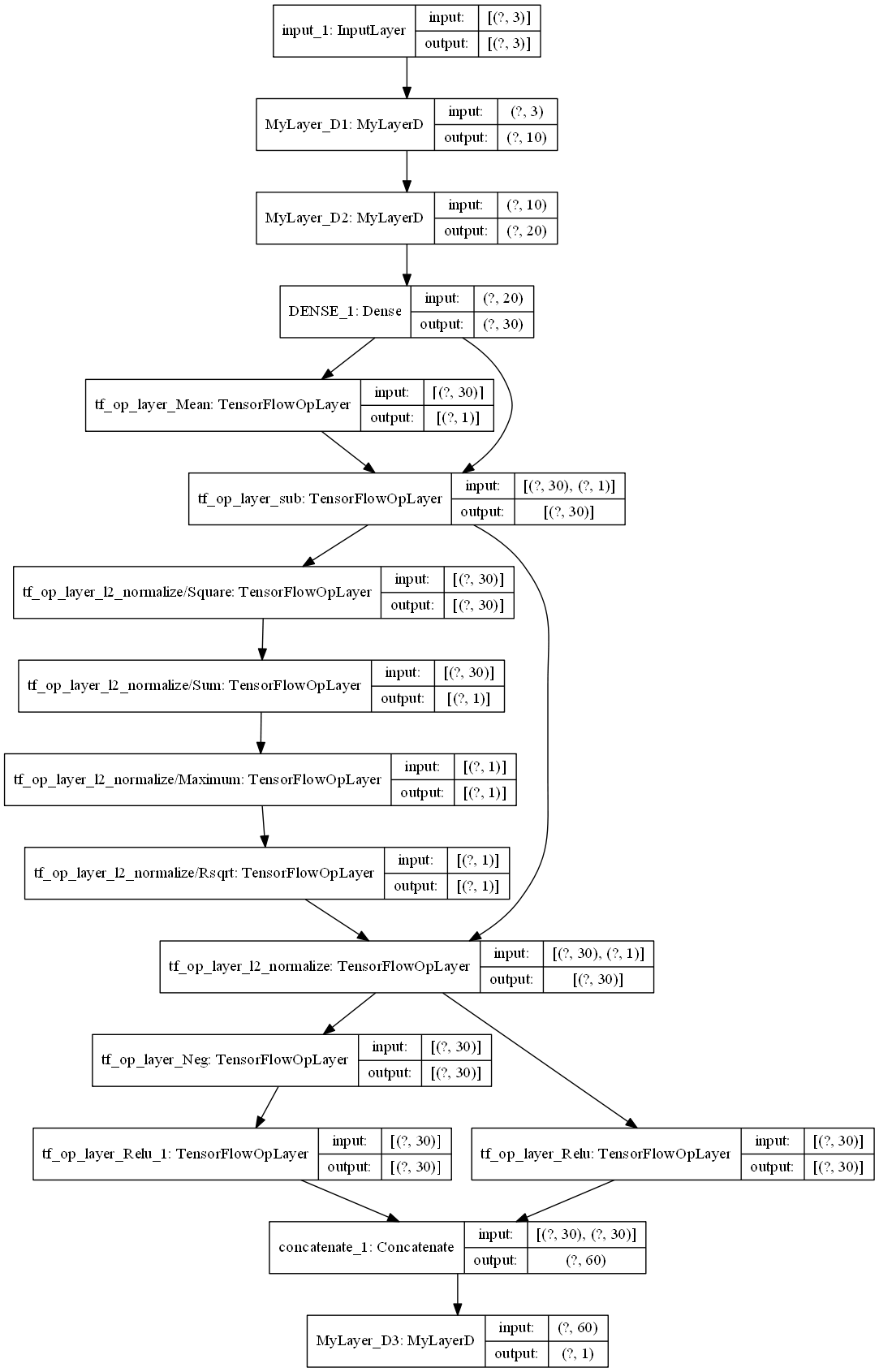
# Custom MLP
class MyModelMLP(tf.keras.Model):
    def __init__(self, input_shape, **kwargs):
        super().__init__(**kwargs)

        self.mylayer1 = MyLayerD(10, tf.nn.relu, name='MyLayer_D1')  # Custom layer
        self.mylayer2 = MyLayerD(20, tf.nn.relu, name='MyLayer_D2')  # Custom layer
        self.layer1 = tf.keras.layers.Dense(30, activation='relu', name='DENSE_1')   # Built in full connectivity layer
        self.mylayer3 = MyLayerD(1, tf.nn.relu, name='MyLayer_D3')  # Custom layer

        # Parameters of the model
        self.input_layer = tf.keras.layers.Input(input_shape)
        self.out = self.call(self.input_layer)
        super().__init__( inputs=self.input_layer,outputs=self.out,**kwargs)

    # Initialize the parameters of the model
    def build(self):
        self._is_graph_network = True
        self._init_graph_network(inputs=self.input_layer,outputs=self.out)

    # Define forward passing of model
    def call(self, inputdata):
        x = self.mylayer1(inputdata)
        x = self.mylayer2(x)
        x = self.layer1(x)
        x = lambda_layer(x)  # Custom Lambda layer
        output = self.mylayer3(x)
        return output
2.1 overview of exporting custom models
# Construct input data
x_input2 = tf.range(6.).numpy().reshape(2, 3)
mymodel1 = MyModelMLP(3, name='MyModelMLP')
mymodel1(x_input2)
mymodel1.summary()
Model: "MyModelMLP"
__________________________________________________________________________________________________
Layer (type)                    Output Shape         Param #     Connected to
==================================================================================================
input_1 (InputLayer)            [(None, 3)]          0
__________________________________________________________________________________________________
MyLayer_D1 (MyLayerD)           (None, 10)           40          input_1[0][0]
__________________________________________________________________________________________________
MyLayer_D2 (MyLayerD)           (None, 20)           220         MyLayer_D1[0][0]
__________________________________________________________________________________________________
DENSE_1 (Dense)                 (None, 30)           630         MyLayer_D2[0][0]
__________________________________________________________________________________________________
tf_op_layer_Mean (TensorFlowOpL [(None, 1)]          0           DENSE_1[0][0]
__________________________________________________________________________________________________
tf_op_layer_sub (TensorFlowOpLa [(None, 30)]         0           DENSE_1[0][0]
                                                                 tf_op_layer_Mean[0][0]
__________________________________________________________________________________________________
tf_op_layer_l2_normalize/Square [(None, 30)]         0           tf_op_layer_sub[0][0]
__________________________________________________________________________________________________
tf_op_layer_l2_normalize/Sum (T [(None, 1)]          0           tf_op_layer_l2_normalize/Square[0
__________________________________________________________________________________________________
tf_op_layer_l2_normalize/Maximu [(None, 1)]          0           tf_op_layer_l2_normalize/Sum[0][0
__________________________________________________________________________________________________
tf_op_layer_l2_normalize/Rsqrt  [(None, 1)]          0           tf_op_layer_l2_normalize/Maximum[
__________________________________________________________________________________________________
tf_op_layer_l2_normalize (Tenso [(None, 30)]         0           tf_op_layer_sub[0][0]
                                                                 tf_op_layer_l2_normalize/Rsqrt[0]
__________________________________________________________________________________________________
tf_op_layer_Neg (TensorFlowOpLa [(None, 30)]         0           tf_op_layer_l2_normalize[0][0]
__________________________________________________________________________________________________
tf_op_layer_Relu (TensorFlowOpL [(None, 30)]         0           tf_op_layer_l2_normalize[0][0]
__________________________________________________________________________________________________
tf_op_layer_Relu_1 (TensorFlowO [(None, 30)]         0           tf_op_layer_Neg[0][0]
__________________________________________________________________________________________________
concatenate_1 (Concatenate)     (None, 60)           0           tf_op_layer_Relu[0][0]
                                                                 tf_op_layer_Relu_1[0][0]
__________________________________________________________________________________________________
MyLayer_D3 (MyLayerD)           (None, 1)            61          concatenate_1[0][0]
==================================================================================================
Total params: 951
Trainable params: 951
Non-trainable params: 0
__________________________________________________________________________________________________
2.2 structure of output custom model
tf.keras.utils.plot_model(mymodel1, to_file='mymodel1.png', show_shapes=True,
                          show_layer_names=True,rankdir='TB', dpi=100, expand_nested=True)
3 application example of user defined model
Please refer to Content of day 4.
from tensorflow.keras.datasets import mnist
mnistdata = mnist.load_data()
(train_features, train_labels), (test_features, test_labels) = mnistdata
# normalization
trainfeatures = train_features / 255
testfeatures = test_features / 255
# Tile
train_fea = trainfeatures.reshape(-1, 784)
test_fea = testfeatures.reshape(-1, 784)
 # Using lambda to build a slightly more complex layer: the back correction layer
def lambda_layer(x, y):
    return tf.keras.layers.concatenate([x, y], axis=1)
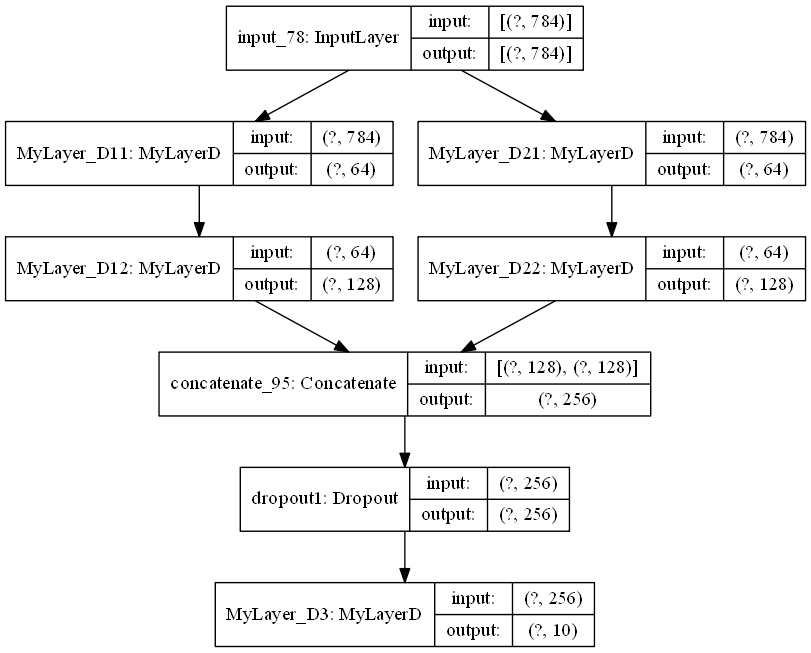
tf.keras.backend.set_floatx('float64')
# Custom MLP
class MyMODEL(tf.keras.Model):
    def __init__(self, input_shape, **kwargs):
        super().__init__(**kwargs)

        self.mylayer11 = MyLayerD(64, tf.nn.relu, name='MyLayer_D11')  # Custom layer
        self.mylayer12 = MyLayerD(128, tf.nn.relu, name='MyLayer_D12')  # Custom layer


        self.mylayer21 = MyLayerD(64, tf.nn.relu, name='MyLayer_D21')  # Custom layer
        self.mylayer22 = MyLayerD(128, tf.nn.relu, name='MyLayer_D22')  # Custom layer


        self.dropout1 = tf.keras.layers.Dropout(0.5, name='dropout1') # Built in layer, discard layer, prevent over fitting
        self.mylayer3 = MyLayerD(10, tf.nn.softmax, name='MyLayer_D3')  # Custom layer


        # Parameters of the model
        self.input_layer = tf.keras.layers.Input(input_shape)
        self.out = self.call(self.input_layer)

        super().__init__( inputs=self.input_layer,outputs=self.out, **kwargs)

    # Initialized model parameters
    def build(self):
        self._is_graph_network = True
        self._init_graph_network(inputs=self.input_layer,outputs=self.out)

    # Define forward passing of model
    def call(self, inputdata, **kwargs):

        x1 = self.mylayer11(inputdata)
        x1 = self.mylayer12(x1)


        x2 = self.mylayer21(inputdata)
        x2 = self.mylayer22(x2)


        x = lambda_layer(x1, x2)  # Lambda custom layer

        x = self.dropout1(x)

        output = self.mylayer3(x)

        return output
mymodel2 = MyMODEL(784, name='MyModelMLP')
mymodel2(train_fea)
mymodel2.summary()
Model: "MyModelMLP"
__________________________________________________________________________________________________
Layer (type)                    Output Shape         Param #     Connected to
==================================================================================================
input_78 (InputLayer)           [(None, 784)]        0
__________________________________________________________________________________________________
MyLayer_D11 (MyLayerD)          (None, 64)           50240       input_78[0][0]
__________________________________________________________________________________________________
MyLayer_D21 (MyLayerD)          (None, 64)           50240       input_78[0][0]
__________________________________________________________________________________________________
MyLayer_D12 (MyLayerD)          (None, 128)          8320        MyLayer_D11[0][0]
__________________________________________________________________________________________________
MyLayer_D22 (MyLayerD)          (None, 128)          8320        MyLayer_D21[0][0]
__________________________________________________________________________________________________
concatenate_95 (Concatenate)    (None, 256)          0           MyLayer_D12[0][0]
                                                                 MyLayer_D22[0][0]
__________________________________________________________________________________________________
dropout1 (Dropout)              (None, 256)          0           concatenate_95[0][0]
__________________________________________________________________________________________________
MyLayer_D3 (MyLayerD)           (None, 10)           2570        dropout1[0][0]
==================================================================================================
Total params: 119,690
Trainable params: 119,690
Non-trainable params: 0
__________________________________________________________________________________________________
tf.keras.utils.plot_model(mymodel2, to_file='mymodel2.png', show_shapes=True,
                          show_layer_names=True, rankdir='TB', dpi=100, expand_nested=True)
Epoch = 50  # Number of iterations of the model
Batch_Size = 128  # Number of samples for batch training
Out_Class = 10  # The number of output categories, 0-9, 10 categories in total
# Model compilation
mYMODEL = MyMODEL(784)
mYMODEL.compile(optimizer='Sgd', loss='categorical_crossentropy', metrics=['accuracy'])
train_label_cate = tf.keras.utils.to_categorical(train_labels, 10)
testlabels = tf.keras.utils.to_categorical(test_labels, 10)
import os

checkpoint_path = "./cp-{val_accuracy:.5f}.ckpt"
checkpoint_dir = os.path.dirname(checkpoint_path)

# Create a callback to ensure the maximum accuracy of the validation dataset
cp_callback = tf.keras.callbacks.ModelCheckpoint(filepath=checkpoint_path,
                                                 save_weights_only=True,
                                                 monitor='val_accuracy',
                                                 mode='max',
                                                 verbose=2,
                                                 save_best_only=True)

# Dynamic change of learning rate: used in model callback
def scheduler(epoch):  # Dynamically changing the parameters of learning rate according to epoch
    if epoch < 10:
        return 0.13
    else:
        return 0.13 * tf.math.exp(0.1 * (10 - epoch))

lr_back = tf.keras.callbacks.LearningRateScheduler(scheduler)
mYMODEL.fit(train_fea, train_label_cate, batch_size=Batch_Size,
            epochs=Epoch, verbose=2, validation_split=0.1,
            callbacks=[cp_callback, lr_back])
Train on 54000 samples, validate on 6000 samples
Epoch 1/50

Epoch 00001: val_accuracy improved from -inf to 0.92200, saving model to ./cp-0.92200.ckpt
54000/54000 - 4s - loss: 0.9787 - accuracy: 0.6990 - val_loss: 0.2899 - val_accuracy: 0.9220
Epoch 2/50

Epoch 00002: val_accuracy improved from 0.92200 to 0.93950, saving model to ./cp-0.93950.ckpt
54000/54000 - 2s - loss: 0.3452 - accuracy: 0.8996 - val_loss: 0.2039 - val_accuracy: 0.9395
Epoch 3/50

Epoch 00003: val_accuracy improved from 0.93950 to 0.95600, saving model to ./cp-0.95600.ckpt
54000/54000 - 3s - loss: 0.2595 - accuracy: 0.9246 - val_loss: 0.1578 - val_accuracy: 0.9560
Epoch 4/50

Epoch 00004: val_accuracy improved from 0.95600 to 0.96417, saving model to ./cp-0.96417.ckpt
54000/54000 - 3s - loss: 0.2044 - accuracy: 0.9395 - val_loss: 0.1282 - val_accuracy: 0.9642
Epoch 5/50

Epoch 00005: val_accuracy improved from 0.96417 to 0.96900, saving model to ./cp-0.96900.ckpt
54000/54000 - 3s - loss: 0.1720 - accuracy: 0.9496 - val_loss: 0.1132 - val_accuracy: 0.9690
Epoch 6/50

Epoch 00006: val_accuracy improved from 0.96900 to 0.96967, saving model to ./cp-0.96967.ckpt
54000/54000 - 3s - loss: 0.1460 - accuracy: 0.9573 - val_loss: 0.1000 - val_accuracy: 0.9697
Epoch 7/50

Epoch 00007: val_accuracy improved from 0.96967 to 0.97433, saving model to ./cp-0.97433.ckpt
54000/54000 - 3s - loss: 0.1291 - accuracy: 0.9624 - val_loss: 0.0911 - val_accuracy: 0.9743
Epoch 8/50

Epoch 00008: val_accuracy improved from 0.97433 to 0.97450, saving model to ./cp-0.97450.ckpt
54000/54000 - 2s - loss: 0.1140 - accuracy: 0.9657 - val_loss: 0.0855 - val_accuracy: 0.9745
Epoch 9/50

Epoch 00009: val_accuracy improved from 0.97450 to 0.97600, saving model to ./cp-0.97600.ckpt
54000/54000 - 3s - loss: 0.1017 - accuracy: 0.9700 - val_loss: 0.0797 - val_accuracy: 0.9760
Epoch 10/50

Epoch 00010: val_accuracy improved from 0.97600 to 0.97633, saving model to ./cp-0.97633.ckpt
54000/54000 - 3s - loss: 0.0948 - accuracy: 0.9713 - val_loss: 0.0814 - val_accuracy: 0.9763
Epoch 11/50

Epoch 00011: val_accuracy did not improve from 0.97633
54000/54000 - 2s - loss: 0.0848 - accuracy: 0.9748 - val_loss: 0.0832 - val_accuracy: 0.9747
Epoch 12/50

Epoch 00012: val_accuracy improved from 0.97633 to 0.97783, saving model to ./cp-0.97783.ckpt
54000/54000 - 3s - loss: 0.0767 - accuracy: 0.9771 - val_loss: 0.0758 - val_accuracy: 0.9778
Epoch 13/50

Epoch 00013: val_accuracy did not improve from 0.97783
54000/54000 - 2s - loss: 0.0706 - accuracy: 0.9788 - val_loss: 0.0742 - val_accuracy: 0.9777
Epoch 14/50

Epoch 00014: val_accuracy did not improve from 0.97783
54000/54000 - 2s - loss: 0.0641 - accuracy: 0.9808 - val_loss: 0.0746 - val_accuracy: 0.9777
Epoch 15/50

Epoch 00015: val_accuracy improved from 0.97783 to 0.97817, saving model to ./cp-0.97817.ckpt
54000/54000 - 2s - loss: 0.0592 - accuracy: 0.9824 - val_loss: 0.0714 - val_accuracy: 0.9782
Epoch 16/50

Epoch 00016: val_accuracy improved from 0.97817 to 0.97917, saving model to ./cp-0.97917.ckpt
54000/54000 - 2s - loss: 0.0559 - accuracy: 0.9835 - val_loss: 0.0727 - val_accuracy: 0.9792
Epoch 17/50

Epoch 00017: val_accuracy did not improve from 0.97917
54000/54000 - 2s - loss: 0.0530 - accuracy: 0.9843 - val_loss: 0.0689 - val_accuracy: 0.9792
Epoch 18/50

Epoch 00018: val_accuracy improved from 0.97917 to 0.98000, saving model to ./cp-0.98000.ckpt
54000/54000 - 3s - loss: 0.0500 - accuracy: 0.9854 - val_loss: 0.0680 - val_accuracy: 0.9800
Epoch 19/50

Epoch 00019: val_accuracy improved from 0.98000 to 0.98083, saving model to ./cp-0.98083.ckpt
54000/54000 - 3s - loss: 0.0477 - accuracy: 0.9863 - val_loss: 0.0675 - val_accuracy: 0.9808
Epoch 20/50

Epoch 00020: val_accuracy did not improve from 0.98083
54000/54000 - 2s - loss: 0.0459 - accuracy: 0.9862 - val_loss: 0.0681 - val_accuracy: 0.9802
Epoch 21/50

Epoch 00021: val_accuracy did not improve from 0.98083
54000/54000 - 2s - loss: 0.0427 - accuracy: 0.9874 - val_loss: 0.0683 - val_accuracy: 0.9793
Epoch 22/50

Epoch 00022: val_accuracy did not improve from 0.98083
54000/54000 - 2s - loss: 0.0411 - accuracy: 0.9888 - val_loss: 0.0696 - val_accuracy: 0.9797
Epoch 23/50

Epoch 00023: val_accuracy did not improve from 0.98083
54000/54000 - 2s - loss: 0.0406 - accuracy: 0.9880 - val_loss: 0.0676 - val_accuracy: 0.9797
Epoch 24/50

Epoch 00024: val_accuracy improved from 0.98083 to 0.98133, saving model to ./cp-0.98133.ckpt
54000/54000 - 2s - loss: 0.0395 - accuracy: 0.9884 - val_loss: 0.0659 - val_accuracy: 0.9813
Epoch 25/50

Epoch 00025: val_accuracy did not improve from 0.98133
54000/54000 - 2s - loss: 0.0390 - accuracy: 0.9887 - val_loss: 0.0662 - val_accuracy: 0.9803
Epoch 26/50

Epoch 00026: val_accuracy did not improve from 0.98133
54000/54000 - 2s - loss: 0.0368 - accuracy: 0.9895 - val_loss: 0.0664 - val_accuracy: 0.9807
Epoch 27/50

Epoch 00027: val_accuracy did not improve from 0.98133
54000/54000 - 2s - loss: 0.0361 - accuracy: 0.9900 - val_loss: 0.0669 - val_accuracy: 0.9803
Epoch 28/50

Epoch 00028: val_accuracy did not improve from 0.98133
54000/54000 - 2s - loss: 0.0353 - accuracy: 0.9896 - val_loss: 0.0674 - val_accuracy: 0.9807
Epoch 29/50

Epoch 00029: val_accuracy did not improve from 0.98133
54000/54000 - 2s - loss: 0.0346 - accuracy: 0.9900 - val_loss: 0.0665 - val_accuracy: 0.9807
Epoch 30/50

Epoch 00030: val_accuracy did not improve from 0.98133
54000/54000 - 2s - loss: 0.0343 - accuracy: 0.9901 - val_loss: 0.0664 - val_accuracy: 0.9802
Epoch 31/50

Epoch 00031: val_accuracy did not improve from 0.98133
54000/54000 - 2s - loss: 0.0339 - accuracy: 0.9906 - val_loss: 0.0669 - val_accuracy: 0.9812
Epoch 32/50

Epoch 00032: val_accuracy did not improve from 0.98133
54000/54000 - 3s - loss: 0.0337 - accuracy: 0.9903 - val_loss: 0.0676 - val_accuracy: 0.9808
Epoch 33/50

Epoch 00033: val_accuracy improved from 0.98133 to 0.98200, saving model to ./cp-0.98200.ckpt
54000/54000 - 2s - loss: 0.0327 - accuracy: 0.9911 - val_loss: 0.0658 - val_accuracy: 0.9820
Epoch 34/50

Epoch 00034: val_accuracy did not improve from 0.98200
54000/54000 - 2s - loss: 0.0315 - accuracy: 0.9909 - val_loss: 0.0666 - val_accuracy: 0.9812
Epoch 35/50

Epoch 00035: val_accuracy did not improve from 0.98200
54000/54000 - 3s - loss: 0.0320 - accuracy: 0.9907 - val_loss: 0.0660 - val_accuracy: 0.9808
Epoch 36/50

Epoch 00036: val_accuracy did not improve from 0.98200
54000/54000 - 2s - loss: 0.0321 - accuracy: 0.9906 - val_loss: 0.0666 - val_accuracy: 0.9810
Epoch 37/50

Epoch 00037: val_accuracy did not improve from 0.98200
54000/54000 - 2s - loss: 0.0315 - accuracy: 0.9910 - val_loss: 0.0668 - val_accuracy: 0.9817
Epoch 38/50

Epoch 00038: val_accuracy did not improve from 0.98200
54000/54000 - 2s - loss: 0.0312 - accuracy: 0.9915 - val_loss: 0.0668 - val_accuracy: 0.9813
Epoch 39/50

Epoch 00039: val_accuracy did not improve from 0.98200
54000/54000 - 2s - loss: 0.0311 - accuracy: 0.9909 - val_loss: 0.0665 - val_accuracy: 0.9810
Epoch 40/50

Epoch 00040: val_accuracy did not improve from 0.98200
54000/54000 - 2s - loss: 0.0302 - accuracy: 0.9914 - val_loss: 0.0662 - val_accuracy: 0.9817
Epoch 41/50

Epoch 00041: val_accuracy did not improve from 0.98200
54000/54000 - 2s - loss: 0.0304 - accuracy: 0.9916 - val_loss: 0.0666 - val_accuracy: 0.9815
Epoch 42/50

Epoch 00042: val_accuracy did not improve from 0.98200
54000/54000 - 2s - loss: 0.0306 - accuracy: 0.9913 - val_loss: 0.0665 - val_accuracy: 0.9815
Epoch 43/50

Epoch 00043: val_accuracy did not improve from 0.98200
54000/54000 - 3s - loss: 0.0300 - accuracy: 0.9919 - val_loss: 0.0661 - val_accuracy: 0.9820
Epoch 44/50

Epoch 00044: val_accuracy improved from 0.98200 to 0.98217, saving model to ./cp-0.98217.ckpt
54000/54000 - 3s - loss: 0.0305 - accuracy: 0.9920 - val_loss: 0.0662 - val_accuracy: 0.9822
Epoch 45/50

Epoch 00045: val_accuracy did not improve from 0.98217
54000/54000 - 2s - loss: 0.0303 - accuracy: 0.9917 - val_loss: 0.0666 - val_accuracy: 0.9815
Epoch 46/50

Epoch 00046: val_accuracy did not improve from 0.98217
54000/54000 - 3s - loss: 0.0301 - accuracy: 0.9920 - val_loss: 0.0661 - val_accuracy: 0.9817
Epoch 47/50

Epoch 00047: val_accuracy did not improve from 0.98217
54000/54000 - 2s - loss: 0.0291 - accuracy: 0.9921 - val_loss: 0.0663 - val_accuracy: 0.9815
Epoch 48/50

Epoch 00048: val_accuracy did not improve from 0.98217
54000/54000 - 2s - loss: 0.0301 - accuracy: 0.9919 - val_loss: 0.0666 - val_accuracy: 0.9820
Epoch 49/50

Epoch 00049: val_accuracy did not improve from 0.98217
54000/54000 - 2s - loss: 0.0295 - accuracy: 0.9922 - val_loss: 0.0666 - val_accuracy: 0.9813
Epoch 50/50

Epoch 00050: val_accuracy did not improve from 0.98217
54000/54000 - 3s - loss: 0.0301 - accuracy: 0.9917 - val_loss: 0.0666 - val_accuracy: 0.9817


<tensorflow.python.keras.callbacks.History at 0x2ce52908>
# The evaluation model is calculated according to the final parameters of the model
test_loss, test_acc = mYMODEL.evaluate(test_fea, testlabels)

print('Test data set cost:{:.8f},Accuracy{:.8f}%%'. format(test_loss, 100*test_acc))
10000/10000 [==============================] - 0s 45us/sample - loss: 0.0664 - accuracy: 0.9801
 Test data set cost: 0.06635048, accuracy rate 98.01000000%%
# Parameter loading
# The new model structure remains consistent.
model_new = MyMODEL(784)
# It needs to be compiled, and the parameters should be consistent with the original
model_new.compile(optimizer='Sgd', loss='categorical_crossentropy', metrics=['accuracy'])

# Load trained parameters
best_para = tf.train.latest_checkpoint(checkpoint_dir)
print('Optimal parameter file:', best_para)
model_new.load_weights(best_para)
predict_loss, predict_acc = model_new.evaluate(test_fea, testlabels)
print('Use the parameters after training','cost:', predict_loss, 'Accuracy', predict_acc)
The optimal parameter file is as follows: cp-0.98217.ckpt
10000/10000 [==============================] - 1s 57us/sample - loss: 0.0663 - accuracy: 0.9800
 The parameter cost after training: 0.066284800849457, accuracy 0.98
click Get more project source code. Welcome Follow, thank Star!!! Scan the WeChat official account pythonfan, get more.