Decision Tree Picks Out Good Watermelons

1. ID3 Algorithmic Theory

(1) algorithm core

The core of the ID3 algorithm is to select the partitioned features based on the information gain and then build the decision tree recursively

(2) Feature selection

Feature selection means selecting the optimal partition attribute and selecting a feature from the features of the current data as the partition criterion for the current node. As the partitioning process continues, it is expected that the branch nodes of the decision tree contain samples of the same category as possible, that is, the "purity" of the nodes increases.

(3) entropy

Entropy represents the degree of uncertainty in a transaction, that is, the amount of information (in general, the amount of information is large, that is, there are too many uncertainties behind this time). The formula for entropy is as follows: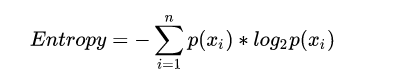

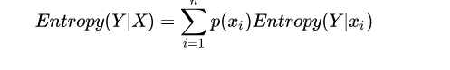
For the conditional entropy of Y under X, it refers to the amount of information (uncertainty) of the variable Y after the information of X. The formula is as follows:

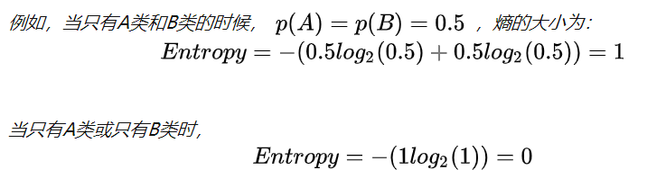
So when Entropy is 1 at its maximum, it is the least effective state for classification, and when it is 0 at its minimum, it is the fully classified state. Because zero is ideal, in general, the entropy is between 0 and 1.

The continuous minimization of entropy is actually the process of improving the classification accuracy.

(4) information gain

Information Gain: Changes in information before and after partitioning a dataset. Calculating the information gain obtained by partitioning a dataset with each eigenvalue is the best option to achieve the highest information gain.

Defines that the information gain of attribute A to dataset D is infoGain(D|A), which is equal to the entropy of D itself, minus the conditional entropy of D under given A, that is:

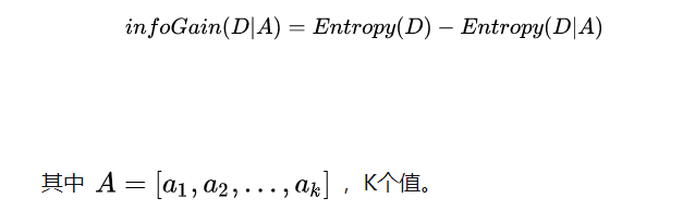
Meaning of information gain: How much less uncertainty has been reduced in original dataset D since attribute A was introduced.

Calculate the information gain after each attribute is introduced, and select the attribute that brings the greatest information gain to D, that is, divide the attribute optimally. Generally, the greater the information gain, the greater the "purity enhancement" resulting from partitioning using attribute A.

(5) Steps

Starting from the root node, the information gain of all possible features is calculated, and the feature with the largest information gain is selected as the partition feature of the nodes.
The sub-nodes are built by different values of the feature.
Then the decision tree is constructed by recursive steps 1-2 for the child nodes.
The final decision tree is obtained until no features can be selected or the categories are identical.

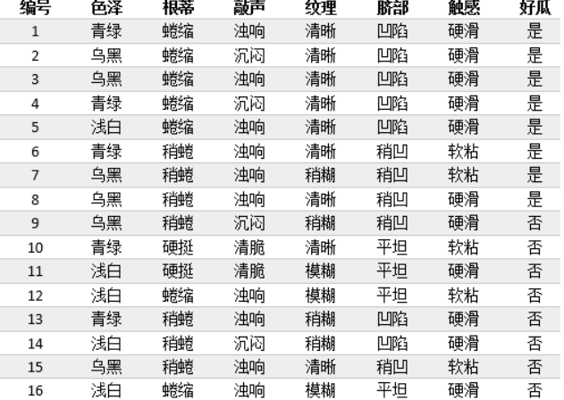
3. Examples of ID3 algorithm application--watermelon tree

(1) Deduction of watermelon tree theory

1. Building decision tree model for watermelon samples

(2) algorithm code

1. Create a watermlon.ipynb file

2. Importing python modules

import pandas as pd
import numpy as np
from collections import Counter
from math import log2

3. Data Acquisition and Processing Functions

#Data Acquisition and Processing
def getData(filePath):
    data = pd.read_excel(filePath)
    return data

def dataDeal(data):
    dataList = np.array(data).tolist()
    dataSet = [element[1:] for element in dataList]
    return dataSet

4. Get property names and category Tags

#Get property name
def getLabels(data):
    labels = list(data.columns)[1:-1]
    return labels
#Get category Tags
def targetClass(dataSet):
    classification = set([element[-1] for element in dataSet])
    return classification

5. Leaf Node Marker

#Branch nodes are marked as leaf nodes, and classes with the largest number of samples are selected as class markers
def majorityRule(dataSet):
    mostKind = Counter([element[-1] for element in dataSet]).most_common(1)
    majorityKind = mostKind[0][0]
    return majorityKind

6. Computing information entropy

#Computing information entropy
def infoEntropy(dataSet):
    classColumnCnt = Counter([element[-1] for element in dataSet])
    Ent = 0
    for symbol in classColumnCnt:
        p_k = classColumnCnt[symbol]/len(dataSet)
        Ent = Ent-p_k*log2(p_k)
    return Ent

7. Building Subdatasets

#Subdataset Construction
def makeAttributeData(dataSet,value,iColumn):
    attributeData = []
    for element in dataSet:
        if element[iColumn]==value:
            row = element[:iColumn]
            row.extend(element[iColumn+1:])
            attributeData.append(row)
    return attributeData

8. Calculate Information Gain

def infoGain(dataSet,iColumn):
    Ent = infoEntropy(dataSet)
    tempGain = 0.0
    attribute = set([element[iColumn] for element in dataSet])
    for value in attribute:
        attributeData = makeAttributeData(dataSet,value,iColumn)
        tempGain = tempGain+len(attributeData)/len(dataSet)*infoEntropy(attributeData)
        Gain = Ent-tempGain
    return Gain

9. Choose the best attribute

#Select Optimal Attribute                
def selectOptimalAttribute(dataSet,labels):
    bestGain = 0
    sequence = 0
    for iColumn in range(0,len(labels)):#Excluding the last category column
        Gain = infoGain(dataSet,iColumn)
        if Gain>bestGain:
            bestGain = Gain
            sequence = iColumn
        print(labels[iColumn],Gain)
    return sequence

10. Set up a decision tree

#Establishing decision trees
def createTree(dataSet,labels):
    classification = targetClass(dataSet) #Get Category Category Category (Collection Weighting)
    if len(classification) == 1:
        return list(classification)[0]
    if len(labels) == 1:
        return majorityRule(dataSet)#Return categories with more sample types
    sequence = selectOptimalAttribute(dataSet,labels)
    print(labels)
    optimalAttribute = labels[sequence]
    del(labels[sequence])
    myTree = {optimalAttribute:{}}
    attribute = set([element[sequence] for element in dataSet])
    for value in attribute:
        
        print(myTree)
        print(value)
        subLabels = labels[:]
        myTree[optimalAttribute][value] =  \
                createTree(makeAttributeData(dataSet,value,sequence),subLabels)
    return myTree

def main():
    filePath = 'watermalon.xls'
    data = getData(filePath)
    dataSet = dataDeal(data)
    labels = getLabels(data)
    myTree = createTree(dataSet,labels)
    return myTree

mytree = main()

Color 1.5798634010685348
 Root pedicle 1.4020814027560324
 Knock 1.3328204045850205
 Texture 1.4466479595102761
 Umbilical 1.5485652260309184
 Touch 0.8739810481273587
 Good melon 0.9975025463691161
['Color and lustre', 'Root pedicle', 'stroke', 'texture', 'Umbilical Cord', 'Touch', 'Melon']
{'Color and lustre': {}}
plain
 Root pedicle 1.3709505944546687
 Knock 1.3709505944546687
 Texture 1.3709505944546687
 Umbilical 0.9709505944546686
 Touch 0.7219280948873621
 Good melon 0.7219280948873621
['Root pedicle', 'stroke', 'texture', 'Umbilical Cord', 'Touch', 'Melon']
{'Root pedicle': {}}
Curl up a little
{'Root pedicle': {'Curl up a little': nan}}
Stiff
{'Root pedicle': {'Curl up a little': nan, 'Stiff': nan}}
Coiled
 Knock 0.0
 Texture 0.9182958340544894
 Umbilical 0.9182958340544894
 Touch 0.9182958340544894
 Good melon 0.9182958340544894
['stroke', 'texture', 'Umbilical Cord', 'Touch', 'Melon']
{'texture': {}}
clear
{'texture': {'clear': nan}}
vague
 Knock 0.0
 Umbilical 0.0
 Touch 1.0
 Good melon 0.0
['stroke', 'Umbilical Cord', 'Touch', 'Melon']
{'Touch': {}}
Soft sticky
{'Touch': {'Soft sticky': nan}}
Hard Slide
{'Color and lustre': {'plain': {'Root pedicle': {'Curl up a little': nan, 'Stiff': nan, 'Coiled': {'texture': {'clear': nan, 'vague': {'Touch': {'Soft sticky': nan, 'Hard Slide': nan}}}}}}}}
Dark green
 Root pedicle 1.4591479170272448
 Knock 1.4591479170272448
 Texture 0.9182958340544896
 Umbilical 1.4591479170272448
 Touch 0.9182958340544896
 Hot melon 1.0
['Root pedicle', 'stroke', 'texture', 'Umbilical Cord', 'Touch', 'Melon']
{'Root pedicle': {}}
Curl up a little
 Knock 0.0
 Texture 1.0
 Umbilical 1.0
 Touch 1.0
 Hot melon 1.0
['stroke', 'texture', 'Umbilical Cord', 'Touch', 'Melon']
{'texture': {}}
clear
{'texture': {'clear': nan}}
Slightly blurry
{'Root pedicle': {'Curl up a little': {'texture': {'clear': nan, 'Slightly blurry': nan}}}}
Stiff
{'Root pedicle': {'Curl up a little': {'texture': {'clear': nan, 'Slightly blurry': nan}}, 'Stiff': nan}}
Coiled
 Knock 0.9182958340544894
 Texture 0.9182958340544894
 Umbilical 0.9182958340544894
 Touch 0.0
 Good melon 0.9182958340544894
['stroke', 'texture', 'Umbilical Cord', 'Touch', 'Melon']
{'stroke': {}}
Turbid Sound
{'stroke': {'Turbid Sound': nan}}
Depressed
 Texture 1.0
 Umbilical 1.0
 Touch 0.0
 Hot melon 1.0
['texture', 'Umbilical Cord', 'Touch', 'Melon']
{'texture': {}}
clear
{'texture': {'clear': nan}}
Slightly blurry
{'Color and lustre': {'plain': {'Root pedicle': {'Curl up a little': nan, 'Stiff': nan, 'Coiled': {'texture': {'clear': nan, 'vague': {'Touch': {'Soft sticky': nan, 'Hard Slide': nan}}}}}}, 'Dark green': {'Root pedicle': {'Curl up a little': {'texture': {'clear': nan, 'Slightly blurry': nan}}, 'Stiff': nan, 'Coiled': {'stroke': {'Turbid Sound': nan, 'Depressed': {'texture': {'clear': nan, 'Slightly blurry': nan}}}}}}}}
Black
 Root Pedicle 0.9182958340544896
 Knock 0.9182958340544896
 Texture 0.9182958340544896
 Umbilical 0.9182958340544896
 Touch 0.9182958340544896
 Good melon 0.9182958340544896
['Root pedicle', 'stroke', 'texture', 'Umbilical Cord', 'Touch', 'Melon']
{'Root pedicle': {}}
Curl up a little
 Knock 0.8112781244591329
 Texture 1.0
 Umbilical 0.0
 Touch 1.0
 Hot melon 1.0
['stroke', 'texture', 'Umbilical Cord', 'Touch', 'Melon']
{'texture': {}}
clear
 Knock 0.0
 Umbilical 0.0
 Touch 1.0
 Hot melon 1.0
['stroke', 'Umbilical Cord', 'Touch', 'Melon']
{'Touch': {}}
Soft sticky
{'Touch': {'Soft sticky': nan}}
Hard Slide
{'texture': {'clear': {'Touch': {'Soft sticky': nan, 'Hard Slide': nan}}}}
Slightly blurry
 Knock 1.0
 Umbilical 0.0
 Touch 1.0
 Hot melon 1.0
['stroke', 'Umbilical Cord', 'Touch', 'Melon']
{'stroke': {}}
Turbid Sound
{'stroke': {'Turbid Sound': nan}}
Depressed
{'Root pedicle': {'Curl up a little': {'texture': {'clear': {'Touch': {'Soft sticky': nan, 'Hard Slide': nan}}, 'Slightly blurry': {'stroke': {'Turbid Sound': nan, 'Depressed': nan}}}}}}
Coiled
 Knock 1.0
 Texture 0.0
 Umbilical 0.0
 Touch 0.0
 Good melon 0.0
['stroke', 'texture', 'Umbilical Cord', 'Touch', 'Melon']
{'stroke': {}}
Turbid Sound
{'stroke': {'Turbid Sound': nan}}
Depressed

4. Decision Tree Algorithms

(1) Comparing the improvement points of ID3

The C4.5 algorithm is a classical algorithm for generating decision trees and an extension and optimization of the ID3 algorithm. The C4.5 algorithm improves the ID3 algorithm mainly:

Selecting partition features with information gain ratio overcomes the shortage of information gain selection.
Information Gain Rate has a preference for attributes with fewer available values.
Can handle discrete and continuous attribute types, that is, continuous attributes are discretized;
Ability to process training data with missing attribute values;
Pruning during tree construction;

(2) Feature selection

(3) Information Gain Rate

The information gain criterion has a preference for attributes with a large number of choices. To reduce the possible adverse effects of this preference, the C4.5 algorithm uses the information gain rate to select the optimal partitioning attribute. Gain Rate Formula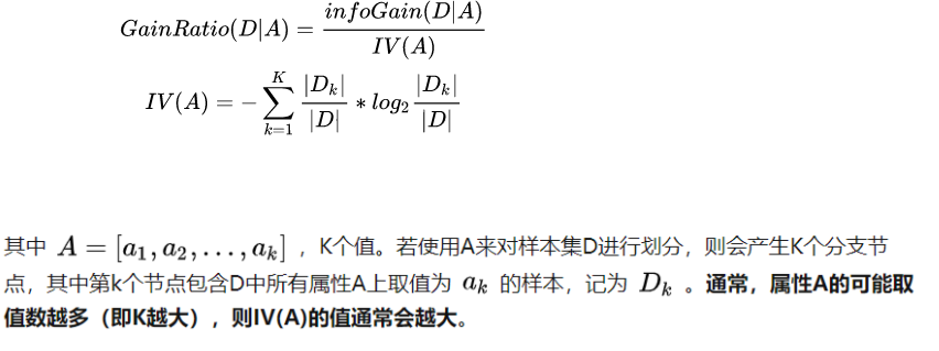
The Information Gain Rate Criterion has a preference for attributes with fewer values available. Therefore, instead of directly selecting the candidate partition attributes with the largest information gain rate, C4.5 first finds out the attributes with higher than average information gain from the candidate partition attributes, and then selects the attributes with the highest information gain rate from them.

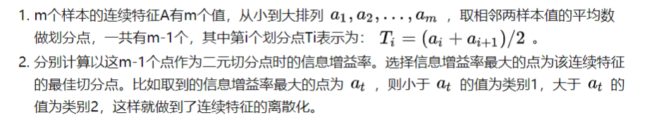
(4) Treatment of continuous features

When the attribute type is discrete, there is no need to discretize the data.

When the attribute type is continuous, the data needs to be discretized. The specific ideas are as follows:

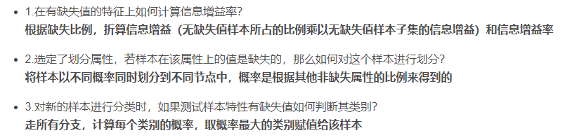
(5) Treatment of missing values

The ID3 algorithm cannot handle missing values, while the C4.5 algorithm can handle missing values (common probability weighting methods). There are three main situations, which are as follows:

V. Summary

This experiment has made me understand the three algorithms ID3, C4.5, CART of decision tree, their advantages and disadvantages, and the differences of improvement. Information gain selection feature is used in ID3, and gain large preference is used. In C4.5, information gain rate is used to select features to reduce the problem of large information gain due to more eigenvalues. The CART classification tree algorithm uses the Gini coefficient to select features. The Gini coefficient represents the model's impurity. The smaller the Gini coefficient, the lower the impurity, the better the features. This is the opposite of the information gain (rate). Experiments were carried out to further understand their respective algorithm implementations.

6. References

https://blog.csdn.net/weixin_46628481/article/details/120911551
https://zhuanlan.zhihu.com/p/139523931
https://zhuanlan.zhihu.com/p/139188759

Keywords: Machine Learning AI Decision Tree

Added by zebrax on Sun, 31 Oct 2021 21:48:26 +0200

Programming VIP

Decision Tree Picks Out Good Watermelons