catalogue
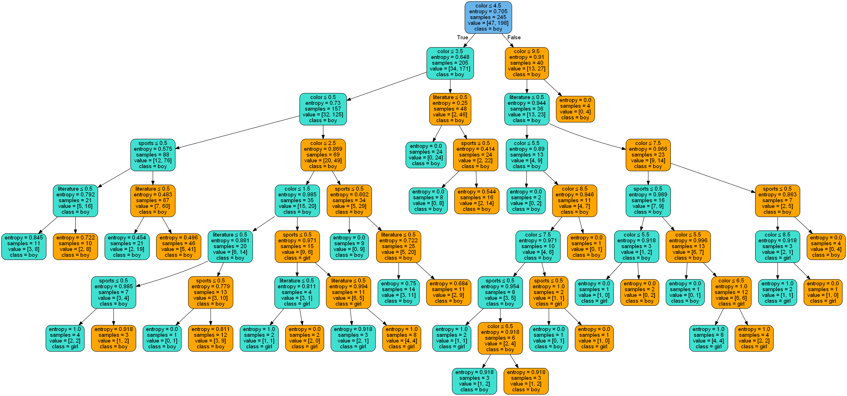
2.1.2 decision tree visualization
2.2 model classification performance prediction
2.2.2 SE, SP and ACC classification performance prediction
2.1 decision tree
2.1.1 sample data set
The total sample data used in this decision tree construction is 351, of which the number of male samples is 283 and the number of female samples is 68; The number of training set samples is 245 and the number of test set samples is 106; Among them, the test intensity accounts for about 30% of the total number of samples.
2.1.2 decision tree visualization
2.2 model classification performance prediction
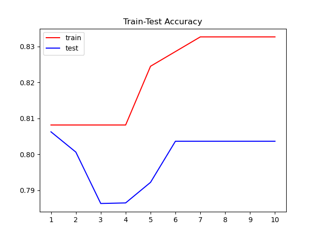
2.2.1 model stability
Performance measurement is an evaluation criterion to measure the generalization ability of the model, which reflects the task requirements; Using different performance measures will often lead to different evaluation results.
Firstly, the score () is used to input the data and labels of the test samples, and the classification score of the model predicted by the test samples is returned;
Step 2: after getting the score, do ten cross validation to see the stability of the model. Using cross in sklearn_ val_ The score function performs cross validation. Input the data characteristics and data labels. Here, cv is set to 10. Perform cross validation for ten times, and the returned test score is also 0.8019. Therefore, it can be seen that the stability of the model is good;
| list | Score |
| Test set | 0.8019 |
| Ten cross validation | 0.8019 |
| Adjust tree depth | 0.8063 |
Step 3: adjust the parameters. This is mainly aimed at the depth of the decision tree. In order to see whether it is over fitting or under fitting, we compare the performance of the training set and the test set. According to table 2.2.1, the result is 0.8063. It can be seen from figure 2.2.1 that there is a tendency of over fitting.
2.2.2 SE, SP and ACC classification performance prediction
In this prediction task, the function predict () in the decision tree is used to predict 106 samples of the test set and return the prediction label of the samples. The evaluation indexes TP, TN, FP and FN of the sample are calculated according to the real marking and prediction results of the test set, and then the evaluation indexes such as SE, SP and ACC are calculated.
The list is as follows, where 1 represents positive class and 0 represents negative class:
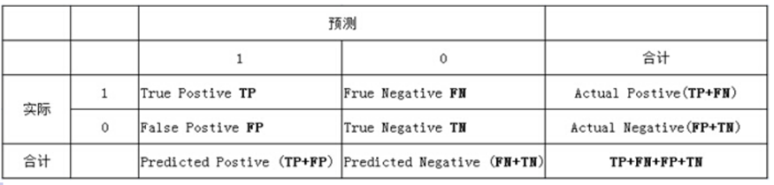
Where TP represents the positive sample with correct prediction; TN represents the negative sample with correct prediction; FP represents the negative sample of prediction error; FN represents a positive sample of prediction errors.
Sensitivity (SE) = TP/(TP+FN) #tpr
Specificity (SP) = TN/(TN+FP) # tnr=1-fpr
Accuracy (ACC) = (TP+TN) / (TP+FP+TN+FN)
The prediction performance of the model is shown in Table 4
| Sensitivity SE | Specific SP | Accuracy ACC |
| 0.942 | 0.300 | 0.821 |
Table 4 performance evaluation of decision tree classification
It can be seen from the table that the ACC accuracy rate shows that 82.1% of the total number of samples can be correctly predicted; According to the sensitivity SE, the prediction accuracy of the model for boys (positive samples) is as high as 94.2%; According to the specific SP, the classification accuracy of the model for girls (negative samples) is only 30%, which may be that the number of girls (negative samples) is too small in the process of model training, resulting in the inaccurate training model, so the accuracy is not high.
#Code implementation
from sklearn.tree import DecisionTreeClassifier
from sklearn.model_selection import train_test_split
from sklearn.model_selection import GridSearchCV
from sklearn.model_selection import cross_val_score
import matplotlib.pyplot as plt
import math
'''
/**************************task1**************************/
2. The decision tree algorithm for division and selection based on information gain rate is realized
 Huan color, like sports, like literature) are classified, and the calculation model predicts performance (package)
contain SE susceptibility=TP/(TP+FN),SP Specificity=TN/(TN+FP),ACC=right/all=(TP+TN)/(TP+FP+TN+FN),The results are illustrated in a friendly way
1.Construction tree step (data processing. Knowledge) classification diagram
2.Prediction performance
/**************************task1**************************/
'''
import pandas as pd
import numpy as np
data = pd.read_csv('data_favorite.txt', header=0, sep=' ')
# data.dropna(how='any', inplace=True)  # type(data)--pandas.core.frame.DataFrame
# Processing non numeric
data["color"] = pd.factorize(data["color"])[0].astype(np.uint16)
# print(data)

# Split data
# First split the data and labels,
X = data.iloc[:, data.columns != "sex"]
y = data.iloc[:, data.columns == "sex"]

# First, convert the data read by pandas into array
X = np.array(X)
y = np.array(y)

# Then divide the data according to the classical 37 points. Because it is randomly selected, the index is chaotic.
from sklearn.model_selection import train_test_split
Xtrain, Xtest, Ytrain, Ytest = train_test_split(X, y, test_size=0.3)
# print('Xtrain:',Xtrain)
# print('Xtest:', Xtest)
# print('Ytrain:',Ytrain)
# print('Ytest:', Ytest)
print(len(Xtrain))
print(len(Xtest))
# Fix the index of test set and training set
'''
for i in [Xtrain, Xtest, Ytrain, Ytest]:
    i.index = range(i.shape[0])
'''

# Train the model. After getting the score, do ten cross validation to see the stability of the model
clf = DecisionTreeClassifier(random_state=25)
clf = clf.fit(Xtrain, Ytrain)

#Calculate the evaluation index according to the real value and predicted value
def performance(labelArr, predictArr):  # Samples must be arrays narray Type class label is 1, 0 # labelArr[i] real category, predictArr[i] predicted category
    # labelArr[i] is actual value,predictArr[i] is predict value
    TP = 0.; TN = 0.; FP = 0.; FN = 0.
    for i in range(len(labelArr)):
        if labelArr[i] == 1 and predictArr[i] == 1:
            TP += 1.
        elif labelArr[i] == 1 and predictArr[i] == 0:
            FN += 1.
        elif labelArr[i] == 0 and predictArr[i] == 1:
            FP += 1.
        elif labelArr[i] == 0 and predictArr[i] == 0:
            TN += 1.
    SE = TP / (TP + FN)  # Sensitivity = TP/P  and P = TP + FN
    SP = TN / (FP + TN) # Specificity = TN/N  and N = TN + FP
    # MCC = (TP * TN - FP * FN) / math.sqrt((TP + FP) * (TP + FN) * (TN + FP) * (TN + FN))
    ACC = (TP + TN) / (TP + TN + FP + FN)
    return SE, SP, ACC

predict_label = clf.predict(Xtest)
print(predict_label)
# print(type(predict_label))
print('Ytest:', Ytest)
# print(type(Ytest))

print(performance(Ytest, predict_label))  # The label of the test set feature judged by the decision tree and the actual label of the test set are input into performance
score_ = clf.score(Xtest, Ytest)
print('Training test scores:', score_)  # Ten cross validation

# Ten cross validation
score = cross_val_score(clf, X, y, cv=10).mean()
print('Ten cross validation:', score_)

# Adjust parameters
# Start with max_depth. In order to see whether it is over fitting or under fitting, it is better to compare the performance of the training set and the test set.
tr = []
te = []
for i in range(10):
    clf = DecisionTreeClassifier(random_state=25, max_depth=i+1,
                                 criterion="entropy")
    clf = clf.fit(Xtrain, Ytrain)
    score_tr = clf.score(Xtrain,Ytrain)
    score_te = cross_val_score(clf,X,y,cv=10).mean()
    tr.append(score_tr)
    te.append(score_te)
print(max(te))
plt.plot(range(1,11),tr,color="red",label="train")
plt.plot(range(1,11),te,color="blue",label="test")
plt.xticks(range(1,11))
plt.legend()
plt.title('Train-Test Accuracy')
plt.savefig(" Decision Tree Train-test Accuracy")
plt.show()
'''
'''
from sklearn import tree
tree.plot_tree(clf)
plt.show()
# Visual decision tree
import graphviz
clf = DecisionTreeClassifier(random_state=25, max_depth=i+1, criterion="entropy")
clf = clf.fit(Xtrain, Ytrain)

tree.export_graphviz(clf, out_file='tree.dot')
data_feature_names = ['color', 'sports', 'literature']
# Visualize data
dot_data = tree.export_graphviz(clf,
                                out_file=None,
                                feature_names=data_feature_names,
                                class_names=['girl', 'boy'],
                                filled=True,
                                rounded=True,
                                special_characters=True)
import pydotplus
graph = pydotplus.graph_from_dot_data(dot_data)

colors = ('turquoise', 'orange')
import collections
edges = collections.defaultdict(list)

for edge in graph.get_edge_list():
    edges[edge.get_source()].append(int(edge.get_destination()))

for edge in edges:
    edges[edge].sort()
    for i in range(2):
        dest = graph.get_node(str(edges[edge][i]))[0]
        dest.set_fillcolor(colors[i])

graph.write_png('tree.png')