In the previous two sections, we can realize some binary classification problems through a simple multilayer neural network, but in some cases, our samples may need to be divided into more than one class, so how to find the current samples in so many classification types is the most likely problem we need to solve.
A very simple idea is to calculate the value of each classification according to the previous Sigmoid method, and then calculate the percentage of each classification value in the total. In this way, according to this proportion, we can find the most likely classification results in a variety of classification types. This is the principle of activating the function Softmax. The most important significance of Softmax is to convert the output values of multiple classifications into probability distributions between [0,1] and 1. Its function is expressed as follows:
Where i represents the ith sample and n is the number of species to be classified.
The matlab implementation of Softmax is as follows:
function y = Softmax(x)
    ex = exp(x);
    y = ex/sum(ex);
end
Next, we can use the activation method of Softmax as the processing method of the output layer to solve the multi classification problem. Let's continue with the previous training. The training function code is as follows:
function [W1,W2] = MultiClass(W1,W2,X,D)
    alpha = 0.9;%Learning factor
    N = 5;%Output classification number
    for k = 1:N
        x = reshape(X(:,:,k),25,1);%Add picture 5*5 Matrix conversion to 25*1 Vector to facilitate training
        d = D(k,:)';

        v1 = W1*x;
        y1 = Sigmoid(v1);%Hidden layer output result, i.e. output layer input

        v = W2*y1;
        y = Softmax(v);%Multi classification problem adoption softmax Function to get the classification result with the greatest probability

        e = d-y;
        delta = e;%If the cross entropy learning rule is not used, it can be changed to y.*(1-y).*e

        e1 = W2'*delta;
        delta1 = y1.*(1-y1).*e1;%Back propagation algorithm, back extrapolation, hidden layer error

        %Update weights for a round of training
        dW1 = alpha*delta1*x';
        W1 = W1+dW1;
        dW2 = alpha*delta*y1';
        W2 = W2+dW2;
    end
end
In order to test the classification effect of our model, let's use a simple 5 * 5 digital matrix as the training set to train our network, and then replace individual elements of the digital matrix as the test set to test the effect of our model.
The following is the code for training with the training set. The classification effect of the training set is d (initialized label matrix).
clc;clear all
X = zeros(5,5,5);%5 The page matrix stores five values
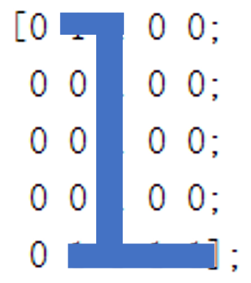
X(:,:,1) = [0 1 1 0 0; %Number 1
0 0 1 0 0;
0 0 1 0 0;
0 0 1 0 0;
0 1 1 1 1];
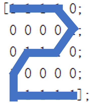
X(:,:,2) = [1 1 1 1 0; %Number 2
0 0 0 0 1;
0 1 1 1 0;
1 0 0 0 0;
1 1 1 1 1];
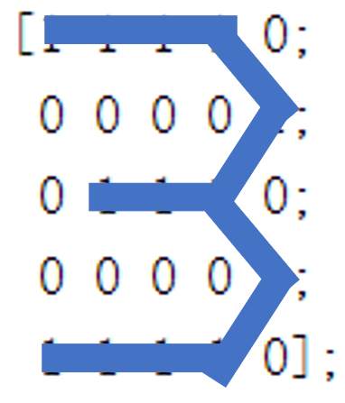
X(:,:,3) = [1 1 1 1 0; %Number 3
0 0 0 0 1;
0 1 1 1 0;
0 0 0 0 1;
1 1 1 1 0];
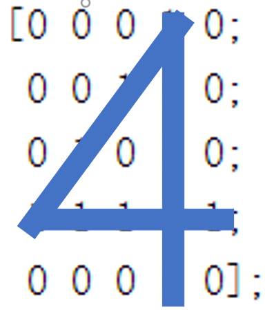
X(:,:,4) = [0 0 0 1 0; %Number 4
0 0 1 1 0;
0 1 0 1 0;
1 1 1 1 1;
0 0 0 1 0];
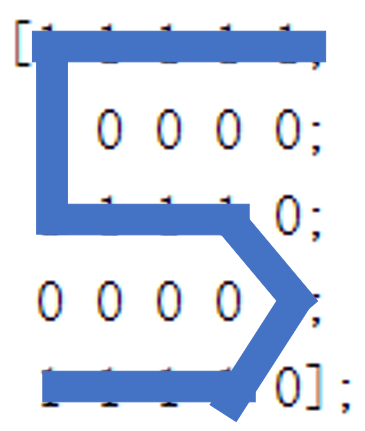
X(:,:,5) = [1 1 1 1 1; %Number 5
1 0 0 0 0;
1 1 1 1 0;
0 0 0 0 1;
1 1 1 1 0];
D = [1 0 0 0 0; %label
0 1 0 0 0;
0 0 1 0 0;
0 0 0 1 0;
0 0 0 0 1];
%Random initialization weight
W1 = 2*rand(50,25)-1;
W2 = 2*rand(5,50)-1;
%train
for epoch = 1:100000
[W1,W2] = MultiClass(W1,W2,X,D);
end
%Training set size
N = 5;
%Test the classification of the training set
for k = 1:N
x = reshape(X(:,:,k),25,1);
v1 = W1*x;
y1 = Sigmoid(v1);
v = W2*y1;
y = Softmax(v)
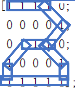
endIn order to test the classification effect of our model, we appropriately transform the previous digital matrix, and then conduct classification test again. The change of digital matrix is shown in the following figure:
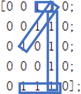
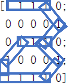
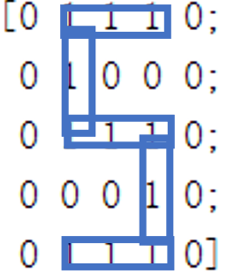
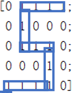
The classification of such a digital matrix only needs to initialize the matrix after training, and then input five pictures into the model.
%% train
TestMultiClass;

%% Initialize 5 pictures
%slightly

%% test
N = 5;
for k = 1:N
    x = reshape(X(:,:,k),25,1);
    v1 = W1*x;
    y1 = Sigmoid(v1);
    v = W2*y1;
    y = Softmax(v)
end
The final result is:
y1 =

    0.0362
    0.0035
    0.0001
    0.9600
    0.0002


y2 =

    0.0000
    0.9984
    0.0015
    0.0000
    0.0000


y3 =

    0.0000
    0.0197
    0.9798
    0.0000
    0.0004


y4 =

    0.4006
    0.0453
    0.4961
    0.0111
    0.0468


y5 =

    0.0034
    0.0248
    0.0077
    0.0010
    0.9631
It can be found that pictures 2, 3 and 5 can be classified accurately, which is similar to our visual perception and obtains the same results.
The test result of picture 1 is the number 4. We may intuitively think that the picture is more like 1, but for the computer, it does not know the content meaning of these shapes, so it can only be classified simply and roughly by calculating the matrix similarity, Therefore, we can also find that the arrangement of matrix elements in Figure 1 is more similar to that in Figure 4.
Similarly, for Figure 4, the above conclusion is more intuitive, but the obvious Figure 5 shape is classified as 1 or 3, which is obviously inconsistent with the result.
The solution to this situation is to increase our training set to avoid the above over fitting. In fact, the training process of real neural network needs thousands of training samples, so the training we conducted above is unscientific and imprecise. If there are too few samples, it is very easy to fit. In the process of preliminary practice, I simply carried out such unscientific training, but such mistakes can also make us actually experience the whole process of neural network establishment and training test, and get some expected results, which can enable us to find the cause and finally solve the problem after discovering the problem.
Therefore, when we actually train the model, we need to collect relevant data. Only a large number of samples can achieve our expected effect.