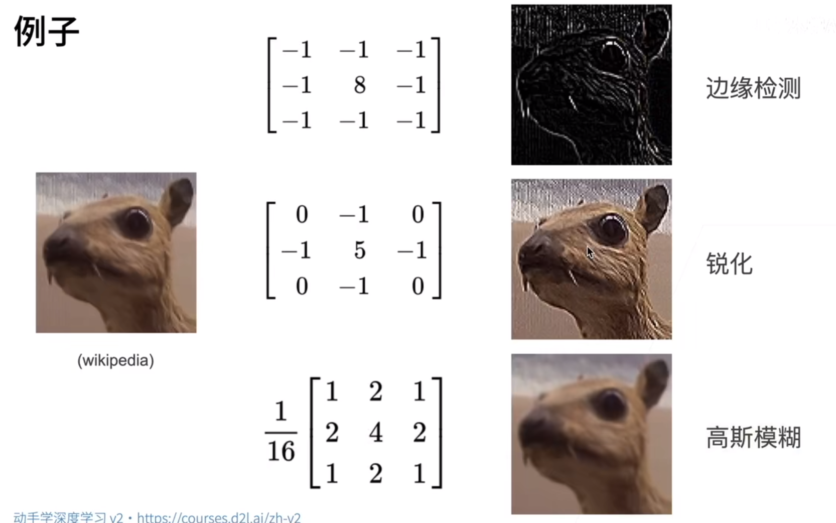
In a word, convolution layer is actually a kind of filter. It makes sense to enlarge its interest and reduce its uninteresting.

 

Mathematical representation of a two-dimensional convolution layer:

 

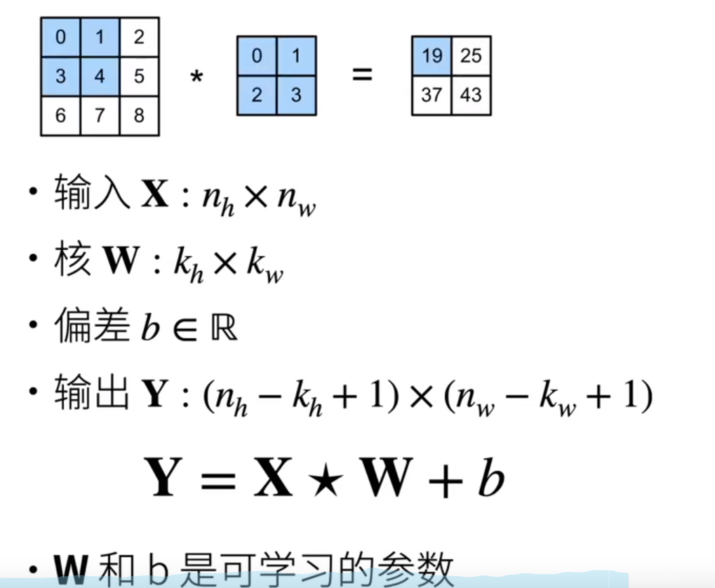
The W here is actually the kernel, the parameter that you learned here in this way, and what you see is a matrix. b is deviation and acts on Y by broadcasting mechanism.

 

 

Two-dimensional crossover and two-dimensional convolution are just one flip away:

 

 

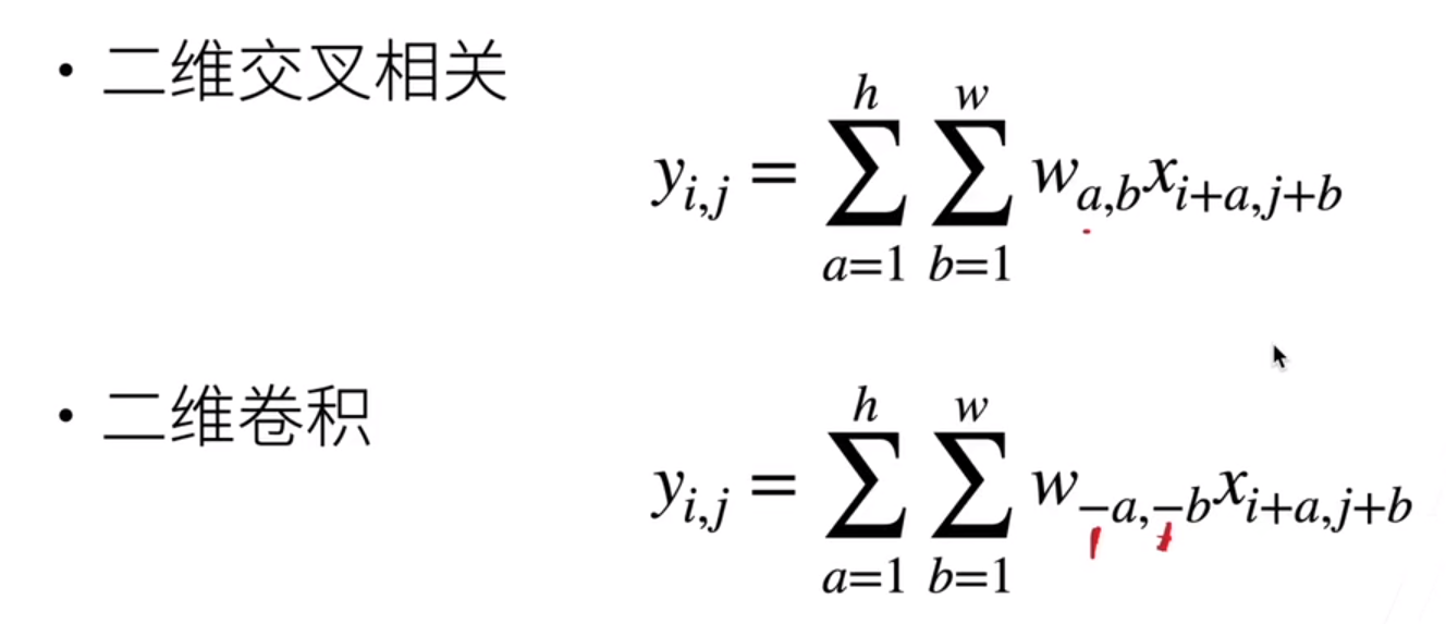
For simplicity, we delete the minus sign. So in neural networks, although we say convolution, we are actually doing cross correlation.

 

Two-dimensional convolution layers are commonly used in image processing, but one and three dimensions are also important in applications.

One-dimensional convolution:

Text, Language, Time Series

Two-dimensional convolution:

Videos, medical images, weather maps

 

Convolution layers cross-correlate the input with the kernel matrix and, after offset, output.

Kernel matrices and offsets are learnable quantities.

The size of the kernel matrix is a hyperparameter.

 

Q&A:

1. Kernel size is mainstream 3x3, up to 5x5. The field of perception is not as big as it is better. Finally, although we can see the whole picture, like why deep learning is more than wide learning, we do less with large nucleus and more with small nucleus, which is the same workload, but a smaller field of vision is better.

 

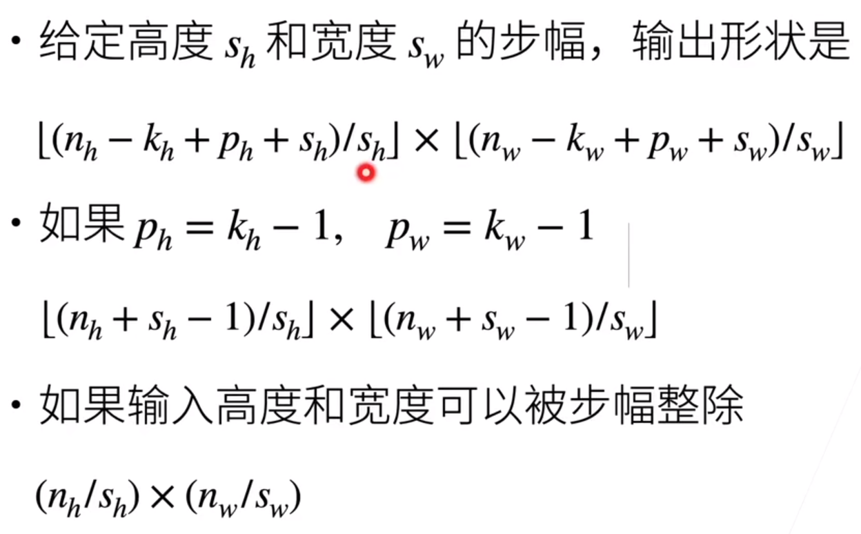
Superparameters for convolution layer controlling output size: fill and step

Fill: You can control how much the output shape is reduced

Step: output shape can be reduced by multiples

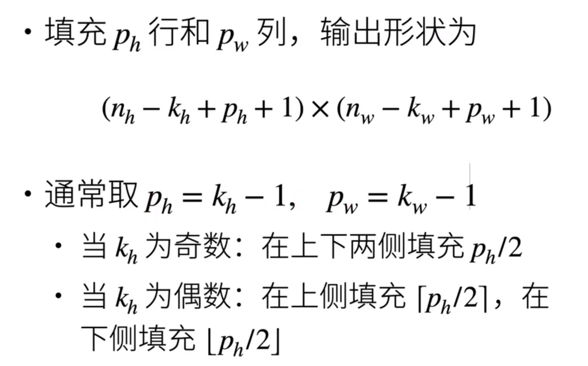
Fill: Add additional rows or columns around the input

Fill is often used to keep the output the same size as the input

　　　　

Step: refers to the step length of the sliding row/column, the height and width can be different

Step calculation:

　　　　

 

 

Q&A:

1. Generally speaking, filling makes the output and input unchanged because it is easier to calculate, otherwise you need to keep thinking about the relationship between input and output changes.

2. Generally speaking, steps are often equal to 1 unless the amount of calculation is significantly too large;

3. The length of the convolution edge is usually odd, because filling is more convenient and symmetrical. But the effect is that parity is almost there.

4. Machine learning is essentially information filtering, information compression, our information has always been lost, as long as it is in operation, it is losing information. We just zoom in on the features we're interested in while compressing.

5. A specific convolution layer is to match a specific texture.

 

The code is as follows:

 1 import torch
 2 from torch import nn
 3 from d2l import torch as d2l
 4 
 5 
 6 # Define an operation for calculating two-dimensional correlation
 7 def corr2d(X,K):
 8     h,w=K.shape
 9     Y=torch.zeros((X.shape[0]-h+1,X.shape[1]-w+1))
10     for i in range(Y.shape[0]):
11         for j in range(Y.shape[1]):
12             Y[i,j]=(X[i:i+h,j:j+w]*K).sum()
13     return Y
14 
15 
16 X = torch.tensor([[0.0, 1.0, 2.0], [3.0, 4.0, 5.0], [6.0, 7.0, 8.0]])
17 K = torch.tensor([[0.0, 1.0], [2.0, 3.0]])
18 print(corr2d(X, K))
19 
20 
21 # Implementing two-dimensional convolution layer
22 class Conv2D(nn.Module):
23     def __init__(self,kernel_size):
24         super().__init__()
25         self.weight=nn.Parameter(torch.rand(kernel_size))
26         self.bias=nn.Parameter(torch.zeros(1))
27 
28     def forward(self,x):
29         return corr2d(x,self.weight)+self.bias
30 
31 
32 # Easy to use: detecting edges of different colors in an image
33 X=torch.ones((6,8)) #z A matrix with two vertical edges is made
34 X[:,2:6]=0
35 print(X)
36 K=torch.tensor([[1.0,-1.0]])
37 Y=corr2d(X,K)
38 print(corr2d(X,K))
39 
40 # # Analogue as an operator to detect vertical edges
41 # X=torch.ones((10,8)) #z makes a matrix with two vertical edges
42 # X[3:7,:]=0
43 # print(X)
44 # K=torch.tensor([[1.0],[-1.0]])
45 # print(corr2d(X,K))
46 
47 # Learning by X Generated Y Convolution Kernel of
48 conv2d=nn.Conv2d(1,1,kernel_size=(1,2),bias=False)
49 X=X.reshape((1,1,6,8))  #Converts a two-dimensional picture into four dimensions, the first is the channel, the second is the sample dimension (number of samples), and the third is the length and width.
50 Y=Y.reshape(1,1,6,7)
51 
52 for i in range(10):
53     Y_hat=conv2d(X)
54     l=(Y_hat-Y)**2
55     conv2d.zero_grad()
56     l.sum().backward()
57     conv2d.weight.data[:]-=3e-2*conv2d.weight.grad
58     if(i+1)%2==0:
59         print(f'batch {i+1}, loss {l.sum():.3f}')
60 
61 print(conv2d.weight.data.reshape((1,2)))# No reshape Will output four dimensions
62 
63 
64 # 2 Dimension becomes 4-D for the following functions
65 XX=torch.zeros((2,3))
66 print(XX)
67 XX=XX.reshape((1,1)+XX.shape)
68 print(XX)
69 
70 # Fill and Step
71 def comp_conv2d(conv2d,X):
72     X=X.reshape((1,1)+X.shape)  #2 Dimension to 4-Dimension
73     Y=conv2d(X)
74     return Y.reshape(Y.shape[2:])
75 
76 conv2d=nn.Conv2d(1,1,kernel_size=3,padding=1) # Fill 1, one row for top, bottom, left, and right
77 X=torch.rand(size=(8,8))
78 print(comp_conv2d(conv2d,X).shape)
79 
80 conv2d=nn.Conv2d(1,1,kernel_size=(5,3),padding=(2,1)) # Front up and down, rear left and right
81 print(comp_conv2d(conv2d,X).shape)
82 
83 conv2d=nn.Conv2d(1,1,kernel_size=3,padding=1,stride=2) # Step 2
84 X=torch.rand(size=(8,8))
85 print(comp_conv2d(conv2d,X).shape)
86 
87 conv2d=nn.Conv2d(1,1,kernel_size=(3,5),padding=(0,1),stride=(3,5)) # Fill 1, one row for top, bottom, left, and right
88 X=torch.rand(size=(8,8))
89 print(comp_conv2d(conv2d,X).shape)