preface
Thesis Name: (ICIP2017) single simple online and realtime tracking with a deep association metric
Thesis address: https://arxiv.org/abs/1703.07402
Open source address: https://github.com/nwojke/deep_sort
catalogue
1, Common multi-target tracking workflow
2, Prerequisite knowledge: Sort multi-target tracking
3, DeepSort multi-target tracking
4, Kalman filter - tracking scene definition
4.1 # Kalman filter - prediction phase
4.2 # Kalman filter - update phase
5, Hungarian matching - tracking scene definition
5.1 Hungarian matching - Mahalanobis distance correlation motion state
5.2 Hungarian matching - cosine distance associated appearance features
5.3 Hungarian matching - complementary
6, Cascade matching - tracking scene
7, IOU matching - tracking scenario
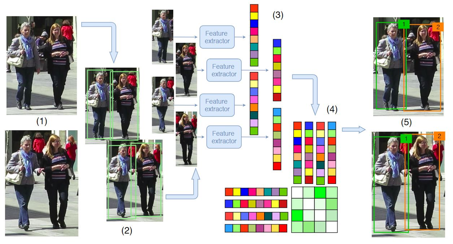
1, Common multi-target tracking workflow
(1) The original frame of a given video;
(2) Running the object detector to obtain the bounding box of the object;
(3) For each detected object, different features are calculated, usually visual and motion features;
(4) Then, the similarity calculation step calculates the probability that the two objects belong to the same target;
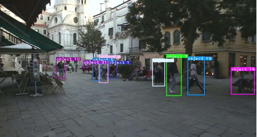
(5) Finally, the association step assigns a numeric ID to each object.
2, Prerequisite knowledge: Sort multi-target tracking
Four core steps

It takes the IOU between "each detection frame" and "all prediction frames of existing targets" as the measurement index of the target relationship between the previous and subsequent frames.
Algorithm core
- The prediction and updating process of Kalman filter.
- Matching process.
Among them, Kalman filter can predict the position of the current time based on the position of the target in front of the time. The Hungarian algorithm can tell us whether a target in the current frame is the same as a target in the previous frame.
Advantages: fast target tracking speed of Sort algorithm; High accuracy without occlusion.
Disadvantages: it hardly handles object occlusion, resulting in a high number of ID switch es; In the case of occlusion, the accuracy is very low.
3, DeepSort multi-target tracking
Background: DeepSort is an improvement based on Sort target tracking. It introduces a deep learning model to extract the appearance features of the target for nearest neighbor matching in the process of real-time target tracking.
Objective: to improve the effect of target tracking under occlusion; At the same time, it also reduces the problem of target ID jump.
Core idea: use recursive Kalman filter and frame by frame Hungarian data association.
4, Kalman filter - tracking scene definition
It is assumed that the tracking scene is defined in the 8-dimensional state space (u, v, γ, h, ẋ, ẏ, γ̇, ḣ), frame center (u, v), aspect ratio γ, Height h and their respective velocities in the image coordinate system.
The uniform motion model is still used here, and (u, v, γ, h) As a direct observation of the object state.

In target tracking, the following two states of the target need to be estimated:
4.1 # Kalman filter - prediction phase

The state transition matrix F is as follows:

• step 2: then use the a posteriori estimated covariance of the previous time k-1 to calculate the a posteriori estimated covariance of the current time K

A priori estimated mean x and covariance P at the current time are estimated by a posteriori estimated mean and variance at the previous time
The implementation code is as follows:
def predict(self, mean, covariance):
    # mean, covariance is equivalent to the mean and covariance of a posteriori estimation at the previous time

    std_pos = [
        self._std_weight_position * mean[3],
        self._std_weight_position * mean[3],
        1e-2,
        self._std_weight_position * mean[3]]
    std_vel = [
        self._std_weight_velocity * mean[3],
        self._std_weight_velocity * mean[3],
        1e-5,
        self._std_weight_velocity * mean[3]]

    # Initialize noise matrix Q
    motion_cov = np.diag(np.square(np.r_[std_pos, std_vel]))

    # x' = Fx
    mean = np.dot(self._motion_mat, mean)

    # P' = FPF^T + Q
    covariance = np.linalg.multi_dot((
        self._motion_mat, covariance, self._motion_mat.T)) + motion_cov

    # Returns the a priori estimated mean x and covariance P at the current time
    return mean, covariance
4.2 # Kalman filter - update phase
- step1: firstly, the Kalman gain matrix K is calculated by using a priori estimation covariance matrix P, observation matrix H and measurement state covariance matrix R

- Step 2: then project the a priori estimated value x of the Kalman filter into the measurement space through the observation matrix H, and calculate the residual y with the measured value z


- Step 3: the predicted value and measured value of Kalman filter are fused according to the proportion of Kalman gain to obtain the a posteriori estimated value x

- Step 4: calculate the a posteriori estimation covariance of Kalman filter

Kalman filter update phase, code implementation:
def update(self, mean, covariance, measurement):

    # The mean and covariance of a priori estimation are mapped to the detection space to obtain Hx 'and HP'
    projected_mean, projected_cov = self.project(mean, covariance)

    chol_factor, lower = scipy.linalg.cho_factor(
        projected_cov, lower=True, check_finite=False)

    # Calculate Kalman gain K
    kalman_gain = scipy.linalg.cho_solve(
        (chol_factor, lower), np.dot(covariance, self._update_mat.T).T,
        check_finite=False).T

    # y = z - Hx'
    innovation = measurement - projected_mean

    # x = x' + Ky
    new_mean = mean + np.dot(innovation, kalman_gain.T)

    # P = (I - KH)P'
    new_covariance = covariance - np.linalg.multi_dot((
        kalman_gain, projected_cov, kalman_gain.T))

    # Returns the a posteriori estimated mean x and covariance P at the current time
    return new_mean, new_covariance
To sum up:
In target tracking, the following two states of the target need to be estimated:
Both the predict stage and the update stage are to calculate the estimated mean x# and covariance P of the Kalman filter. The difference is that the former is a priori estimation based on the previous historical state, while the latter is a posteriori estimation that integrates the measured value information and makes correction.
5, Hungarian matching - tracking scene definition
Solving the correlation between the predicted state and the measured state of Kalman filter can be realized by constructing Hungarian matching.
Association of two states
- Kalman filter prediction state, a posteriori results
- Measurement status, detector results.
Two indicators to achieve correlation
- Motion information (calculated by "Mahalanobis distance")
- Appearance characteristics (calculated by "cosine distance")
Finally, the linear weighted sum is used to combine the two indicators.
5.1 Hungarian matching - Mahalanobis distance correlation motion state
Mahalanobis distance, also known as covariance distance, is an effective method to calculate the similarity between two unknown sample sets, which measures the matching degree of prediction and detection. In order to integrate the motion information of the object, the (square) Mahalanobis distance between the predicted state and the measured state is used:

Where, d and y represent measurement distribution and prediction distribution respectively; S is the covariance matrix between two distributions. It is a real symmetric positive definite matrix. Cholesky decomposition can be used to solve the Mahalanobis distance.
Function: Mahalanobis distance estimates the uncertainty of the tracker state by calculating the deviation between the "prediction frame" and the "detection frame".
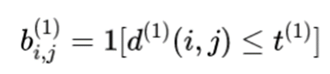
This is an indicator that compares the threshold of Mahalanobis distance and chi square distribution, 9.4877. If the Mahalanobis distance is less than this threshold, it represents a successful match.
Note: since the dimension of the measurement distribution (4-D) is inconsistent with the dimension of the prediction distribution (8-D), the prediction distribution needs to be projected into the measurement space through the observation matrix H (this step is actually to take out the first 4 measurement state variables from the 8 estimated state variables), Code implementation:
# Project state distribution to measurement space.
def project(self, mean, covariance):
    std = [
        self._std_weight_position * mean[3],
        self._std_weight_position * mean[3],
        1e-1,
        self._std_weight_position * mean[3]]

    # Initialize the covariance matrix R of the measurement state
    innovation_cov = np.diag(np.square(std)) # The diagonal matrix is used, and there is no correlation between different dimensions

    # The mean vector is mapped to the detection space to obtain Hx
    mean = np.dot(self._update_mat, mean)

    # The covariance matrix is mapped to the detection space to obtain HP'H^T
    covariance = np.linalg.multi_dot((
        self._update_mat, covariance, self._update_mat.T))

    return mean, covariance + innovation_cov # Plus measurement noise
Calculate Mahalanobis distance, code implementation:
# Compute gating distance between state distribution and measurements.
def gating_distance(self, mean, covariance, measurements,
                    only_position=False):

    # Firstly, the mean and covariance of the predicted state distribution need to be projected into the measurement space
    mean, covariance = self.project(mean, covariance)

    # If only the central position is considered
    if only_position:
        mean, covariance = mean[:2], covariance[:2, :2]
        measurements = measurements[:, :2]

    # cholesky decomposition of covariance matrix
    cholesky_factor = np.linalg.cholesky(covariance)

    # Calculate the pairwise difference between the two distributions
    d = measurements - mean

    # The Mahalanobis distance is calculated by triangular solution
    z = scipy.linalg.solve_triangular(
        cholesky_factor, d.T, lower=True, check_finite=False,
        overwrite_b=True)

    # Return square Mahalanobis distance
    squared_maha = np.sum(z * z, axis=0)
    return squared_maha
5.2 Hungarian matching - cosine distance associated appearance features
Background:
When the uncertainty of object motion state is relatively low, using Mahalanobis distance is indeed a good choice. Because the Kalman filter uses the uniform motion model, it can only provide a relatively rough linear estimation of the moving position of the object. When the object accelerates or decelerates suddenly, the distance between the prediction frame and the detection frame of the tracker will become relatively far. At this time, only using the Mahalanobis distance will become very inaccurate.
Design:
DeepSort also designed a depth appearance feature descriptor for each target, which is actually a 128 dimensional unit feature vector extracted by ReID network trained offline on pedestrian re recognition data set (module length is 1). For each tracker, keep its last 100 appearance feature descriptor sets R successfully associated with the detection frame, and calculate the minimum cosine distance between them and the detection frame:

Then, an appropriate threshold can be set to exclude matches with particularly large differences in appearance features.
ReID network:
Deep Sort adopts Cosine depth feature network trained by large-scale personnel re identification data set, which contains more than 1100000 images of 1261 pedestrians, making it very suitable for depth measurement learning in personnel tracking environment.
Cosine depth feature network uses a wide residual network, which has two convolution layers and six residual blocks. L2 normalization layer can calculate the similarity between different pedestrians to be compatible with cosine appearance measurement. By calculating the cosine distance between pedestrians, the smaller the cosine distance is, the more similar the two pedestrian images are. The network structure of cosine depth feature is shown in the figure below.
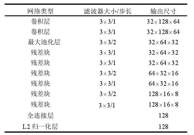
Using Cosine depth feature network parameters, each detection box The inner picture is compressed into a 128 dimensional vector that can best represent the specific information of the picture, and the appearance description vector is obtained after normalization.
Here, the appearance feature vector library is used to save the appearance feature vectors that have been successfully matched recently, and the minimum distance in the de cosine distance during matching can adapt to short-term occlusion. For example, if it is currently occluded, the previous appearance information is used to distinguish. As long as there is a good match in the last 30 frames, the track and detection are matched, which can better reduce the occlusion problem.
Cosine distance is associated with appearance features, which are expanded in detail:
Cosine distance is used to measure the distance between apparent features. A 128 dimensional vector is extracted from reid model, and cosine distance is used for comparison:
 Is cosine similarity, and cosine distance = 1-cosine similarity. Cosine distance is used to measure the apparent features of Kalman prediction and the corresponding apparent features of detector, so as to predict ID more accurately. Only using motion information for matching in SORT will lead to serious ID Switch. The introduction of appearance model + cascade matching can alleviate this problem.

As above, an indicator is also used in the cosine distance part. If the cosine distance is less than, it is considered to match. This threshold is set to 0.2 in the code (controlled by the parameter max_dist). This is a super parameter and is generally set to 0.6 in face recognition.
5.3 Hungarian matching - complementary
The two indicators can complement each other to solve different problems of association matching:
On the one hand, Mahalanobis distance can provide information about possible object positions based on motion, which is particularly useful for short-term prediction;
On the other hand, when the discriminant power of motion is weak, the cosine distance will consider the appearance information, which is particularly useful for recovering identity after long-term occlusion.
In order to establish the correlation problem, we use weighted sum to combine the two indicators:
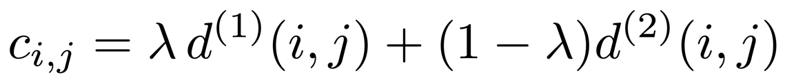
You can use super parameters λ To control the impact of each indicator on the consolidation cost. During the experiment of this paper, it is found that when the camera motion is large, it will λ= 0 is a reasonable choice (only appearance information is used at this time).
6, Cascade matching - tracking scene
When the object is occluded for a long time, Kalman filter can not accurately predict the target state. Therefore, the probability quality is dispersed in the state space, and the peak of observation likelihood is reduced. However, when two trajectories compete for the same detection result, the Mahalanobis distance will bring greater uncertainty. Because it effectively reduces the distance between the standard deviation of any detection and the mean value of the projected trajectory, and may lead to increased trajectory fragmentation and unstable trajectory. Therefore, Deep Sort introduces cascade matching to give priority to targets that appear more frequently. The specific pseudo code of the algorithm is as follows:
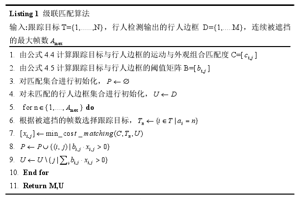
In the cost matrix of cascade matching, the element value is the weighted sum of Mahalanobis distance and cosine distance. Implementation code:
def matching_cascade(
        distance_metric, max_distance, cascade_depth, tracks, detections,
        track_indices=None, detection_indices=None):

    if track_indices is None:
        track_indices = list(range(len(tracks)))
    if detection_indices is None:
        detection_indices = list(range(len(detections)))

    unmatched_detections = detection_indices
    matches = []

    # Traverse different ages
    for level in range(cascade_depth):
        if len(unmatched_detections) == 0:  # No detections left
            break

        # Pick out the tracker corresponding to the age
        track_indices_l = [
            k for k in track_indices
            if tracks[k].time_since_update == 1 + level
        ]
        if len(track_indices_l) == 0:  # Nothing to match at this level
            continue

        # Match the tracker and the unmatched detection box
        matches_l, _, unmatched_detections = \
            min_cost_matching(
                distance_metric, max_distance, tracks, detections,
                track_indices_l, unmatched_detections)
        matches += matches_l

    # Pick out unmatched trackers
    unmatched_tracks = list(set(track_indices) - set(k for k, _ in matches))
    return matches, unmatched_tracks, unmatched_detections
The essence of this matching is to select all confirmed tracks, give priority to matching those younger tracks with unmatched detection frames, and then turn to those older tracks.
This makes it easier for younger trackers to match under the same appearance features and Mahalanobis distance. As for the definition of age, the tracker uses age + 1 each time it predict s.
7, IOU matching - tracking scenario
This stage occurs after cascade matching. The matched tracker objects are unconfirmed tracks and tracks with age 1 in the previous round of cascade matching failure This helps to reduce the probability of appearance changes caused by sudden occlusion in a frame.
# Pick unconfirmed tracks from all trackers
unconfirmed_tracks = [
    i for i, t in enumerate(self.tracks) if not t.is_confirmed()]

# From the trackers that failed in the previous round of cascade matching, select one consecutive frame without matching (equivalent to age=1)
# And unconfirmed_ Add tracks
iou_track_candidates = unconfirmed_tracks + [
    k for k in unmatched_tracks_a if
    self.tracks[k].time_since_update == 1]

# IOU match them with the detections on the remaining unmatched
matches_b, unmatched_tracks_b, unmatched_detections = \
    linear_assignment.min_cost_matching(
        iou_matching.iou_cost, self.max_iou_distance, self.tracks,
        detections, iou_track_candidates, unmatched_detections)
8, Experimental results
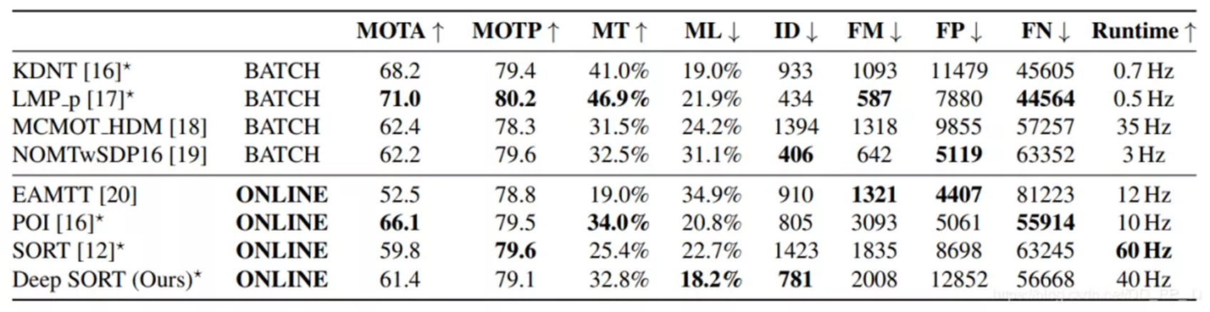
- MOTA, MOTP, MT, ML, FN, ID swiches, FM and other indicators are selected for the evaluation model.
- Compared with sort, the ID Switch index of Deep SORT decreased by 45%, reaching the SOTA at that time. Through experiments, it is found that the MOTA, MOTP, MT, ML and FN indexes of Deep SORT have improved compared with the previous ones.
- There are many FP S, which are mainly caused by too large Detection and Max age.
- The speed reaches 20Hz, half of which is spent on apparent feature extraction.
9, Deep Sort open source code
The Deep Sort algorithm based on YOLO has different versions of open source code on the network. The following three are the Deep Sort multi-target tracking system based on yov5, yov4 and yov3.
[1]YOLOv5+Pytorch+Deep Sort
Open source address: Yolov5_DeepSort_Pytorch
The detection results generated by YOLOv5 are a series of object detection architectures and models pre trained on the COCO data set, which are passed to the Deep Sort multi-target tracking object algorithm.
Development environment:
matplotlib>=3.2.2
numpy>=1.18.5
opencv-python>=4.1.2
Pillow
PyYAML>=5.3.1
scipy>=1.4.1
torch>=1.7.0
torchvision>=0.8.1
tqdm>=4.41.0
seaborn>=0.11.0
pandas
easydict
Model effect:
[2]YOLOv4+TF+Deep Sort
Open source address: Deep-SORT-YOLOv4-tf
Development environment:
# $ conda create --name <env> --file <this file>
# platform: linux-64
imutils=0.5.3=pypi_0
keras=2.3.1=pypi_0
matplotlib=3.2.1=pypi_0
numpy=1.18.4=pypi_0
opencv-python=4.2.0.34=pypi_0
pillow=7.1.2=pypi_0
python=3.6.10=h7579374_2
scikit-learn=0.23.1=pypi_0
scipy=1.4.1=pypi_0
tensorboard=2.2.1=pypi_0
tensorflow=2.0.0=pypi_0
tensorflow-estimator=2.1.0=pypi_0
tensorflow-gpu=2.2.0=pypi_0
Model effect:
[3]YOLOv3+Pytorch+Deep Sort
Open source address: Deep-Sort_pytorch-yolov3
Development environment:
python 3 (python2 not sure)
numpy
scipy
opencv-python
sklearn
torch >= 0.4
torchvision >= 0.1
pillow
vizer
edict
Model effect:
Article reference
[1] Bao Jun, Dong Yachao, Liu Hongzhe Based on deep_ Summary of sort target tracking algorithm Beijing Key Laboratory of information service engineering, Beijing Union University
[2] Zhu Zhenkun, Dai Deyun, Wang Jikai, Chen Zonghai Based on fasterr_ Design of multi - target tracking algorithm based on CNN Department of automation, University of science and technology of China
[3] Xie Jiaxing Research on video multi-target tracking algorithm in crowded scene Zhejiang University
[4] Gu Yanfei Based on improved Yolo_ Research and implementation of V3 + deepsort multi-target tracking system Liaoning University
Online article reference:
Reference 1: https://zhuanlan.zhihu.com/p/97449724
Reference 2: https://yunyang1994.gitee.io/2021/08/27/DeepSort-%E5%A4%9A%E7%9B%AE%E6%A0%87%E8%B7%9F%E8%B8%AA%E7%AE%97%E6%B3%95-SORT-%E7%9A%84%E8%BF%9B%E9%98%B6%E7%89%88/
Reference 3: https://mp.weixin.qq.com/s?__biz=MzA4MjY4NTk0NQ==&mid=2247485748&idx=1&sn=eb0344e1fd47e627e3349e1b0c1b8ada&chksm=9f80b3a2a8f73ab4dd043a6947e66d0f95b2b913cdfcc620cfa5b995958efe1bb1ba23e60100&scene=126&sessionid=1587264986&key=1392818bdbc0aa1829bb274560d74860b77843df4c0179a2cede3a831ed1c279c4603661ecb8b761c481eecb80e5232d46768e615d1e6c664b4b3ff741a8492de87f9fab89805974de8b13329daee020&ascene=1&uin=NTA4OTc5NTky&devicetype=Windows +10+x64&version=62090069&lang=zh_ CN&exportkey=AeR8oQO0h9Dr%2FAVfL6g0VGE%3D&pass_ ticket=R0d5J%2BVWKbvqy93YqUC%2BtoKE9cFI22uY90G3JYLOU0LtrcYM2WzBJL2OxnAh0vLo
Reference 4: https://zhuanlan.zhihu.com/p/80764724
Thesis address: https://arxiv.org/abs/1703.07402
Open source address: https://github.com/nwojke/deep_sort
This article is for your reference only. Thank you. If there are any errors, please point them out~