Delay model of WebRTC video receiving buffer based on Kalman filter

stay WebRTC In the video processing pipeline of, the receiver buffer JitterBuffer is a key component: it is responsible for the out of order rearrangement and framing of RTP packets, RTP packet loss retransmission, requesting retransmission of key frames, estimating buffer delay and other functions. The buffer delay JitterDelay has an important impact on the one-way delay of video stream, which largely determines the real-time performance of the application. This paper does not intend to comprehensively analyze the implementation details of the receiver buffer, but only the calculation of buffer delay JitterDelay

1 Composition of receiver delay

The delay of WebRTC video receiver includes three parts: buffer delay JitterDelay, decoding delay DecodeDelay and rendering delay RenderDelay. Among them, DecodeDelay and RenderDelay are relatively stable, while JitterDelay is greatly affected by the code rate of the sender and network conditions. JitterDelay is also the biggest factor causing the receiver delay

The buffer delay consists of two parts: the delay caused by bit rate burst caused by transmitting large-size video frames and the delay caused by network noise. WebRTC uses Kalman Filter to estimate the network transmission rate and network queuing delay, and then determines the buffer delay. Based on the theoretical study of Kalman Filter, combined with WebRTC source code, this paper deeply analyzes the calculation and update process of buffer delay in detail

2 Kalman filter theory learning

This section mainly refers to references [1] [2] [3], which is used as an introductory material to learn the basic principle of Kalman filter. In short, Kalman filter is an optimized autoregressive data processing algorithm. Literature [2] summarizes the basic idea of Kalman filter:

"Essentially, filtering is a signal processing and transformation (removing or weakening unwanted components and enhancing required components) The process of. Kalman filter belongs to a software filtering method. Its basic idea is to take the minimum mean square error as the best estimation criterion, adopt the state space model of signal and noise, update the estimation of state variables by using the estimated value of the previous time and the observed value of the current time, and obtain the estimated value of the current time. The algorithm estimates the signal to be processed to meet the minimum mean square error according to the established system equation and observation equation. "

The following is a brief analysis of the basic process of Kalman filter based on literature [1]

2.1 establishment of system mathematical model

First, we introduce a discrete control process system. The system can be described by a linear stochastic difference equation:
notes: differential equation, see: How to understand the form of differential equation- Know See cvgmt Your answer

X(K) = AX(K-1) + BU(k) + W(k)          (2.1.1)

Plus the measured value of the system:

Z(k) = HX(k) + V(k)                    (2.1.2)

In the above two equations, X(k) is the system state at time k, and U(k) is the control quantity of the system at time K.
A and B are system parameters. For multi model systems, they are matrices.
Z(k) is the measured value at time k, H is the parameter of the measurement system, and for multi measurement system, H is the matrix.
W(k) and V(k) represent process noise and measurement noise respectively They are assumed to be Gaussian white noise, and their covariances are Q and R, respectively

2.2 Kalman filter process

First, we use the process model of the system to predict the system state of the next state.
Assuming that the current system state is k, according to the process model of the system, the current state can be predicted based on the previous state of the system:

X(k|k-1)=AX(k-1|k-1) + BU(k)          (2.2.1)

In equation (2.2.1), X(k|k-1) is the result predicted by the previous state, X(k-1|k-1) is the optimal result of the previous state, and U(k) is the control quantity of the current state.
So far, our system results have been updated. However, the error covariance corresponding to X(k|k-1) has not been updated. We use P to represent the error covariance:

P(k|k-1)=AP(k-1|k-1)A'+ Q             (2.2.2)

In formula (2.2.2), P(k|k-1) is the error covariance corresponding to X(k|k-1), P(k-1|k-1) is the error covariance corresponding to X(k-1|k-1), A 'represents the transpose matrix of A, and Q is the process noise covariance of the system process. Equations 1 and 2 are the first two of the five formulas of Kalman filter, that is, the prediction of the system

Now we have the predicted value of the current state, and then we collect the measured value of the current state. Combining the predicted and measured values, we can obtain the optimal estimation X(k|k) of the current state (k):

X(k|k) = X(k|k-1) + Kg(k)[Z(k) - HX(k|k-1)] (2.2.3)

Where Kg is Kalman gain:

Kg(k)= P(k|k-1) H'/ (H P(k|k-1) H'+ R)              (2.2.4)

So far, we have obtained the optimal estimate X(k|k) in K state. However, in order to keep the Kalman filter running until the end of the system process, we also need to update the error covariance of X(k|k) in K state:
notes: covariance, see: Mr. Ma explained how to explain the concepts of "covariance" and "correlation coefficient" in a straightforward way- Know

P(k|k)=(I-Kg(k) H) P(k|k-1)                         (2.2.5)

Where I is the identity matrix. When the system enters the k+1 state, P(k|k) is P(k-1|k-1) of equation (2). In this way, the algorithm can continue the autoregressive operation

The above equations 1 ~ 5 are the core algorithm of Kalman filter, including five important steps: prediction value calculation, error covariance calculation, optimal value estimation, Kalman gain calculation, error covariance update and so on

3 calculation process of JitterDelay in webrtc

This section analyzes the calculation process of buffer delay JitterDelay at video receiving end in combination with WebRTC source code

3.1 calculation formula of jitterdelay
According to the analysis in the first section, JitterDelay is caused by two parts: the delay caused by large frame transmission and the delay caused by network noise. The calculation formula is as follows:

JitterDelay = theta[0] * (MaxFS – AvgFS) + [noiseStdDevs * sqrt(varNoise) – noiseStdDevOffset]    (3.1.1)

Where theta[0] is the reciprocal of the channel transmission rate, MaxFS is the maximum frame size received since the beginning of the session, and AvgFS is the average frame size.
notes: divided by the channel transmission rate
Noisestdevs represents the noise coefficient of 2.33,varNoise represents the noise variance, and noisestdevoffset is the noise deduction constant of 30.

Before the decoding thread obtains a frame of video data from the buffer for decoding, it will calculate the buffer delay of the current frame according to formula 3.1.1, and then add the decoding delay and rendering delay to obtain the expected rendering end time of the current frame. Then, according to the current time, the waiting time of the current frame before decoding is determined to ensure the smoothness of video rendering

3.2 update process of jitterdelay

Before the decoding thread obtains a frame of video data from the buffer for decoding, it will update the local state of the buffer according to the size, timestamp and current local time of the current frame, including the maximum frame size, average frame size, average noise value, channel transmission rate, network queuing delay and other parameters. The update process is shown in Figure 1:

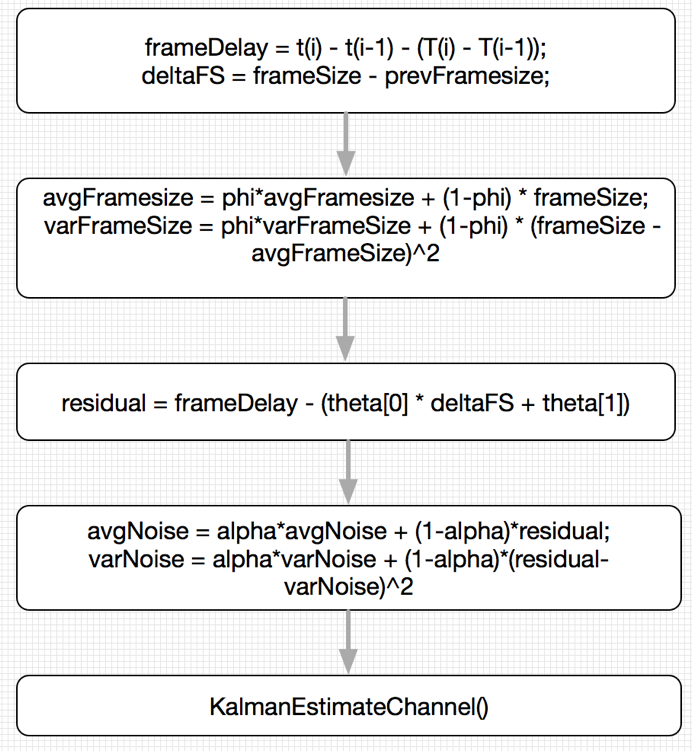
Figure 1 video receiver buffer status update process png

First, determine the inter frame relative delay frameDelay and the inter frame size difference deltaFS:

frameDelay = t(i) – t(i-1) – (T(i) – T(i-1)) (3.2.1)
deltaFS = frameSize – prevFrameSize (3.2.2)

Where t (I) represents the local receiving time of the current frame, and t (i-1) represents the local receiving time of the previous frame; T (I) represents the timestamp of the current frame, and t (i-1) represents the timestamp of the previous frame.
frameDelay indicates the relative delay of two adjacent frames, and frameDelay > 0 indicates that frame i takes longer on the road than frame i-1. frameSize and prevFrameSize represent the size of the current frame and the previous frame respectively

Then calculate the average and variance of the frame size:

avgFrameSize = phi * avgFrameSize + (1-phi) * frameSize (3.2.3)
varFrameSize = phi * varFrameSize + (1-phi) * (frameSize – avgFramesize)^2 (3.2.4)

Next, the delay residual (reflecting the size of network noise) is calculated, and the noise mean and variance are calculated accordingly:

residual = frameDelay – (theta[0] * deltaFSBytes + theta[1]) (3.2.5)
avgNoise = alpha*avgNoise + (1-alpha)*residual (3.2.6)
varNoise = alpha*varNoise + (1 – alpha)*(residual – avgNoise)^2 (3.2.7)
alpha = pow(399/400, 30/fps) (3.2.8)

Where alpha represents the probability coefficient, which is affected by the frame rate fps: when fps becomes low, alpha will become smaller, indicating that the current noise becomes larger, and the noise variance is more affected by the current noise The closer the real-time frame rate is to 30 fps, the better avgNoise represents the average noise since the beginning. theta[0] represents the channel transmission rate and theta[1] represents the network queuing delay

Finally, the Kalman filter dynamically adjusts the channel transmission rate theta[0] and network queuing delay theta[1] according to the current inter frame delay and inter frame size difference. The specific process is discussed in detail in the next section

At this point, the update process of JitterDelay ends.
When the next frame data arrives, use the update result to calculate JitterDelay, and execute the update process again

4 Kalman filter update buffer status

Combined with WebRTC source code, this section deeply analyzes the process of Kalman filter updating channel transmission rate theta[0] and network queuing delay theta[1], which is also the core algorithm of buffer delay estimation

4.1 definition of mathematical symbols

X_bar:  vector X
X_hat:  vector X Estimated value of
X(i):  vector X The first i Components
[x y z]: Include element xyz Row vector of
X_bar^T: vector X_bar Transpose vector of
E{X}:  random variable X Expectations

4.2 theoretical derivation process

d(i) = t(i) – t(i-1) – (T(i) – T(i-1)) (4.2.1)

t(i) represents the local receiving time of the current frame, and t(i-1) represents the local receiving time of the previous frame;
T(i) represents the sampling time of the transmitting end of the current frame, that is, the timestamp, and T(i-1) represents the sampling time of the previous frame.
D (i) > 0 means that frame i takes longer on the road than frame i-1. Equation 4.2.1 is the measured value of the system

d(i) = dL(i) / C(i) + m(i) + v(i) (4.2.2)

dL(i) represents the difference between the length of frame i and frame i-1, C(i) represents the channel transmission rate, m(i) represents the network queuing delay of frame i, v(i) represents the measurement noise, and its covariance is R.
Where [1/C(i) m(i)] is the target value we require, that is, channel transmission rate and network queuing delay Equation 4.2.2 is the predicted value of the system

theta_bar(i) = [1/C(i) m(i)]^T As frame i State column vector;
h_bar(i) = [dL(i) 1]^T Is the inter frame length difference column vector;
theta_bar(i+1) = theta_bar(i) + u_bar(i)； u_bar(i)Indicates process noise;
Q(i) = E{u_bar(i) * u_bar(i)^T} Represents the process noise covariance matrix;
diag(Q(i)) = [10^-13 10^-3]^T Q(i)Is a diagonal matrix;

Estimation process:

theta_hat(i) = [1/C_hat(i) m_hat(i)]^T； // Target estimate
z(i) = d(i) – h_bar(i)^T * theta_hat(i-1)
= d(i) – (dL(i)/C_hat(i-1) + m_hat(i-1)) (4.2.3)

The meaning of the above formula is to estimate the time consumption at this time with the estimated value of the previous time:

dL(i)/C_hat(i-1) + m_hat(i-1)

Then the residual z(i) is calculated from the current observed value d(i) and the estimated value

theta_hat(i) = theta_hat(i-1) + z(i) * k_bar(i) (4.2.4)

The above formula represents the state iteration relationship between time i and time i-1: the state at time i-1 plus the product of the residual z(i) at time i and the Kalman filter at time i, where the kalman gain at time i is calculated as follows:

k_bar(i)=[(E(i-1)+Q(i))*h_bar(i)]/[var_v_hat(i)+h_bar(i)^T*(E(i-1)+Q(i))*h_bar(i)] (4.2.5)
E(i) = (I–k_bar(i)*h_bar(i)^T)*[E(i-1)+Q(i)] (4.2.6)
var_noise(i) = max(alpha*var_noise(i-1)+(1–alpha)*z(i)^2, 1) (4.2.7)
alpha = pow(399 / 400, 30 / fps) (4.2.8)
var_v_hat(i)=(300*exp[-fabs(deltaFS)/maxFrameSize)+1]*sqrt(varNoise) (4.2.9)

Where I is the 2 * 2 unit matrix and E(i) is the error covariance (which is the key parameter of Kalman filter iteration).
var_noise is noise variance, var_v_hat is the filtered average value of noise standard deviation index, which is the measured noise covariance R of frame i,
It has a great influence on the final calculated Kalman gain: var_ v_ When hat (I) is large, the Kalman gain is small, which means that the noise in this measurement is large, and the final estimated value is closer to the last estimated value and less affected by this residual error

4.3 WebRTC code implementation

The following pseudo code is a concise summary of vcmjitterestimator:: Kalman estimatechannel function in WebRTC, and describes the code implementation of Kalman filter

void VCMJitterEstimator::KalmanEstimateChannel(frameDelayMS, deltaFSBytes) {

// Calculate the sum of error covariance and process noise covariance: E = E + Q;

_thetaCov[0][0] += _Qcov[0][0];

_thetaCov[0][1] += _Qcov[0][1];

_thetaCov[1][0] += _Qcov[1][0];

_thetaCov[1][1] += _Qcov[1][1];


// Calculate Kalman gain:

// K = E*h'/(sigma + h*E*h')

// h = [deltaFS 1], Eh = E*h'

// hEh_sigma = h*E*h' + sigma

Eh[0] = _thetaCov[0][0] * deltaFSBytes + _thetaCov[0][1];

Eh[1] = _thetaCov[1][0] * deltaFSBytes + _thetaCov[1][1];

// sigma is the exponential average filtering result of the standard deviation of the measurement noise, that is, the measurement noise covariance R.

double sigma = (300.0 * exp(-fabs(static_cast<double>(deltaFSBytes)) /

(1e0 * _maxFrameSize)) +1) * sqrt(varNoise);

hEh_sigma = deltaFSBytes * Eh[0] + Eh[1] + sigma;

kalmanGain[0] = Eh[0] / hEh_sigma;

kalmanGain[1] = Eh[1] / hEh_sigma;


// Calculate the residual to obtain the optimal estimation

measureRes = frameDelayMS - (deltaFSBytes * _theta[0] + _theta[1]);

_theta[0] += kalmanGain[0] * measureRes;

_theta[1] += kalmanGain[1] * measureRes;


// Update error covariance: E = (I - K*h)*E;

t00 = _thetaCov[0][0]; t01 = _thetaCov[0][1];

_thetaCov[0][0] = (1 - kalmanGain[0] * deltaFSBytes) * t00 -

kalmanGain[0] * _thetaCov[1][0];

_thetaCov[0][1] = (1 - kalmanGain[0] * deltaFSBytes) * t01 -

kalmanGain[0] * _thetaCov[1][1];

_thetaCov[1][0] = _thetaCov[1][0] * (1 - kalmanGain[1]) -

kalmanGain[1] * deltaFSBytes * t00;

_thetaCov[1][1] = _thetaCov[1][1] * (1 - kalmanGain[1]) -

kalmanGain[1] * deltaFSBytes * t01;

}

So far, one iteration of Kalman filter to estimate channel transmission rate and network queuing delay is completed

5 Summary

Based on the theoretical study of the basic principle of Kalman filter, combined with WebRTC source code, this paper deeply analyzes the calculation method and update process of buffer delay at WebRTC video receiver. Through this article, further deepen the learning and understanding of WebRTC.

reference

[1] Principle description of Kalman filter http://blog.sciencenet.cn/blog-1009877-784428.html
[2] Basic principle and application of Kalman filter [J] Software guide, Vol. 8, No. 11, Nov. 2009
[3] An Introduction to the Kalman Filter [J]. University of North Carolina at Chapel Hill Department of Computer Science
Chapel Hill, NC 27599-3175
[4] A Google Congestion Control Algorithm for Real-Time Communication
https://tools.ietf.org/html/draft-alvestrand-rmcat-congestion-03
[5] Analysis and Design of the Google Congestion Control for Web Real-time
Communication[J]. MMSys '16 Article No.13

Keywords: network webrtc

Added by santhosh_89 on Sun, 16 Jan 2022 20:40:59 +0200

Programming VIP