1, SVD basis
Invisible semantic index: one of the earliest applications of SVD is information retrieval. We call the method of using SVD as implicit semantic index (LSI) or invisible semantic analysis (LSA)

Recommender system: another application of SVD is recommender system. The more advanced recommender system first uses SVD to build a subject space from the data, and then calculates the similarity under the space, so as to improve the effect of recommender.

Unlike PCA, SVD decomposes the covariance matrix of data, while SVD decomposes the matrix directly on the original matrix. Moreover, we can decompose the matrix of non square matrix and get the left singular matrix U, sigma matrix Σ and right singular matrix VT.

1.1 basic knowledge of singular value and eigenvalue:
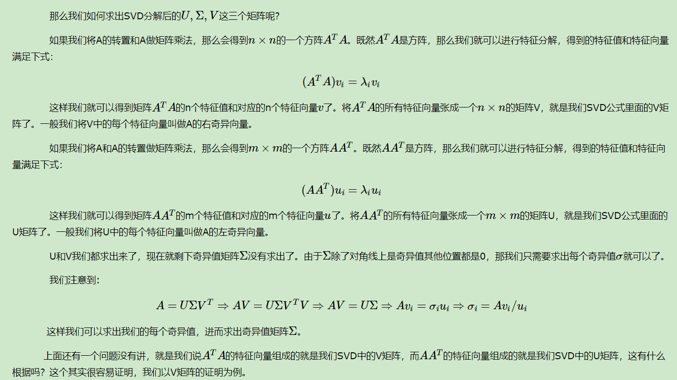
Both eigenvalue decomposition and singular value decomposition are widely used in machine learning. There is a very close relationship between them. I will talk about that the purpose of eigenvalue decomposition and singular value decomposition is the same, which is to extract the most important features of a matrix. Let's talk about eigenvalue decomposition first:

1) Characteristic value:

If A vector v is the eigenvector of square A, it can be expressed in the following form:

In this case, λ is called the eigenvalue corresponding to the eigenvector v. a set of eigenvectors of a matrix is a set of orthogonal vectors. Eigenvalue decomposition is to decompose a matrix into the following forms:

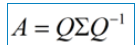
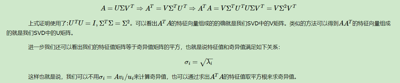
Where Q is the matrix composed of the eigenvectors of matrix A, Σ is a diagonal matrix, and every element on the diagonal is a eigenvalue. I've quoted some references here to illustrate. First of all, it should be clear that a matrix is actually a linear transformation, because the vector obtained by multiplying a matrix by a vector is actually equivalent to a linear transformation of this vector. For example, the following matrix:

In fact, the corresponding linear transformation is in the following form:

Because the result of multiplying matrix M by a vector (x,y) is:

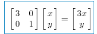
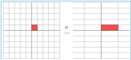
The above matrix is symmetric, so this transformation is a stretching transformation in the direction of x and y axes (each element on the diagonal will stretch and transform a dimension, when the value is > 1, it is stretched, when the value is < 1, it is shortened). When the matrix is not symmetric, if the matrix is like the following:

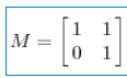
The transformation it describes is as follows:

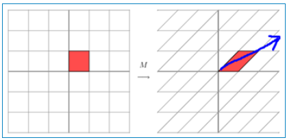
In fact, this is the stretching transformation of an axis on a plane (as shown by the blue arrow). In the figure, the blue arrow is the most important direction of change (there may be more than one direction of change). If we want to describe a transformation, we can describe the main direction of change of the transformation. Looking back at the formula of eigenvalue decomposition before, the sigma matrix obtained by decomposition is a diagonal matrix, in which the eigenvalues are arranged from large to small, and the eigenvector corresponding to these eigenvalues is to describe the change direction of the matrix (from the main change to the secondary change arrangement)

When the matrix is high-dimensional, then the matrix is a linear transformation in high-dimensional space. The linear change may not be represented by pictures, but it can be imagined that the transformation also has many transformation directions. The first N eigenvectors obtained by eigenvalue decomposition correspond to the most important N change directions of the matrix. We can approximate this matrix (transformation) by using the first N change directions. That is to say: extract the most important features of this matrix. To sum up, eigenvalue decomposition can get eigenvalues and eigenvectors. Eigenvalues represent how important the feature is, and eigenvectors represent what the feature is. Each eigenvector can be understood as a linear subspace. We can do many things with these linear subspaces. However, eigenvalue decomposition has many limitations, such as the matrix of transformation must be square matrix.

2, Definition of SVD

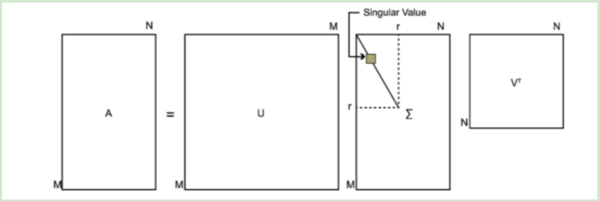
SVD also decomposes the matrix, but unlike eigendecomposition, SVD does not require the matrix to be decomposed to be a square matrix. Suppose that our matrix A is a m × n matrix, then we define the SVD of matrix A as:
A=UΣVT
Where u is a matrix of M × m, Σ is a matrix of M × n, all of them are 0 except the elements on the main diagonal, each element on the main diagonal is called singular value, and V is a matrix of n × n. U and V are unitary matrices, that is to say, UTU=I,VTV=I. The following figure shows the definition of SVD:
　　　　
　　　　


Code implementation SVD:
SCV implementation is related to linear algebra, but we don't need to worry about the implementation of SVD. There is a linear algebra toolbox called linear algebra in Numpy that can help us. Let's demonstrate its usage for a simple matrix

 from numpy import *
from numpy import linalg as la
 
df = mat(array([[1,1],[1,7]]))
U,Sigma,VT = la.svd(df)
print(U)
# [[ 0.16018224  0.98708746]
#  [ 0.98708746 -0.16018224]]
print(Sigma)
# [7.16227766 0.83772234]
print(VT)
# [[ 0.16018224  0.98708746]
#  [ 0.98708746 -0.16018224]]

# (user x Commodity)    # A value of 0 indicates that the user has not evaluated this product, which can be used as a recommended product
def loadExData2():
    return [[0, 0, 0, 0, 0, 4, 0, 0, 0, 0, 5],
            [0, 0, 0, 3, 0, 4, 0, 0, 0, 0, 3],
            [0, 0, 0, 0, 4, 0, 0, 1, 0, 4, 0],
            [3, 3, 4, 0, 0, 0, 0, 2, 2, 0, 0],
            [5, 4, 5, 0, 0, 0, 0, 5, 5, 0, 0],
            [0, 0, 0, 0, 5, 0, 1, 0, 0, 5, 0],
            [4, 3, 4, 0, 0, 0, 0, 5, 5, 0, 1],
            [0, 0, 0, 4, 0, 4, 0, 0, 0, 0, 4],
            [0, 0, 0, 2, 0, 2, 5, 0, 0, 1, 2],
            [0, 0, 0, 0, 5, 0, 0, 0, 0, 4, 0],
            [1, 0, 0, 0, 0, 0, 0, 1, 2, 0, 0]]
 
# Instead of the standest function above, this function uses the reduced dimension matrix of SVD to calculate the score
def svdEst(dataMat, user, simMeas, item):
    n = shape(dataMat)[1]
    simTotal = 0.0; ratSimTotal = 0.0
    U,Sigma,VT = la.svd(dataMat)
    Sig4 = mat(eye(4)*Sigma[:4])  #Transforming singular value vector into singular value matrix
    xformedItems = dataMat.T * U[:,:4] * Sig4.I  # Dimension reduction method transforms items into low dimensional space by U matrix (singular value column is selected for commodity number row x)
    for j in range(n):
        userRating = dataMat[user,j]
        if userRating == 0 or j == item:
            continue
        # Note here: because the reduced dimension matrix is different from the original matrix (the row changes from user to commodity), when comparing two commodities, you should take [all columns in this row] and then transfer it to column vector parameter
        similarity = simMeas(xformedItems[item,:].T,xformedItems[j,:].T)
        # Print (% d is similar to% d in% F% (item, J, similarity))
        simTotal += similarity
        ratSimTotal += similarity * userRating
    if simTotal == 0:
        return 0
    else:
        return ratSimTotal/simTotal
 
# The results were tested as follows:
myMat = mat(loadExData2())
result1 = recommend(myMat,1,estMethod=svdEst)   # Parameter transfer is required to change the default function
print(result1)
result2 = recommend(myMat,1,estMethod=svdEst,simMeas=pearsSim)
print(result2)

SVD applied to pictures:

from skimage import io
import matplotlib.pyplot as plt
 
path = 'male_god.jpg'
data = io.imread(path)
data = mat(data)        # Matrix multiplication can be used in dimension reduction only after mat processing
U,sigma,VT = linalg.svd(data)
# Before reconstruction, according to the previous method, we need to select the singular value that reaches a certain energy degree
cnt = sum(sigma)
print(cnt)
cnt90 = 0.9*cnt    # Singular value at 90%
print(cnt90)
count = 50        # Select the first 50 singular values
cntN = sum(sigma[:count])
print(cntN)
 
# Reconstruction matrix
dig = mat(eye(count)*sigma[:count]) # Get diagonal matrix
# dim = data.T * U[:,:count] * dig.I # Dimension reduction extra variable is useless here
redata = U[:,:count] * dig * VT[:count,:]   # restructure
 
plt.imshow(redata,cmap='gray')  # Ash collection
plt.show()  # You can use the save function to save the picture

The most important calculation steps for SVD are as follows:

Data set dimensionality reduction: the sigma here is a diagonal matrix (the sigma vector returned from the original svd needs to be used to build the matrix, and the count value needs to be used to build the matrix). U is the left singular matrix returned by svd, and count is the number of singular values specified by us, which is also the dimension of the sigma matrix.
Reconstruction of data set: the sigma here is also a diagonal matrix (it needs to use the sigma vector returned by the original svd to build the matrix, and it needs to use the value of count). VT is the right singular matrix returned by svd, and count is the number of singular values we specify (it can be selected according to the rule of 90% energy).

1. SVD for PCA
   Quoted article
   Quoted article