preface

In my last blog, I briefly explained the call of scikit fuzzy, and explained it with a case commonly used by big guys. In recent learning, I found other functions in skfuzzy, including automatic setting and visual display of reference values, which are introduced below.

1, Case description

Similarly, it is the classic two inputs, one output, three reference values and nine rules. Compared with the previous blog, we introduce the membership function of input relative to reference value in detail. And visual display.

2, Automatic setting of reference value and membership function of input attribute

1. Automatic setting of reference value

Compared with the traditional manual setting (the program is as follows), the automatic setting of reference value undoubtedly greatly reduces the entry difficulty of fuzzy reasoning.
The manual setting code is as follows:

# Output set 3 reference values
y['N'] = fuzz.trimf(y_range, [1, 1, 5])
y['M'] = fuzz.trimf(y_range, [1, 5, 10])
y['P'] = fuzz.trimf(y_range, [5, 10, 10])

The automatic setting code is as follows

x_stain.automf(3)  # Set 3 reference values and generate them automatically
x_oil.automf(3)

The number of reference values needs to be set

2. Membership function

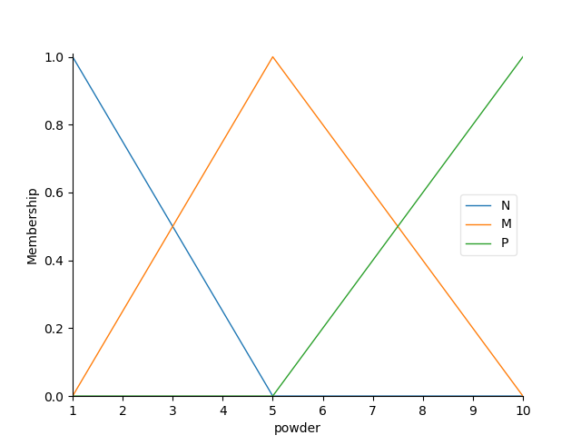
For the output, we set three reference values, using the triangular membership function, in which the three parameter scores correspond to [lower left, upper right and lower right] of the triangular membership function respectively. Its visualization is shown in Figure 1. The visualization procedure is as follows:

# Reference value setting visualization
x_stain.view(), x_oil.view(), y.view()

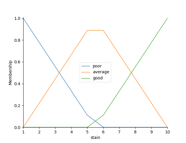
For the two inputs, we use the function of skfuzzy library to generate automatically. In this case, the trapezoidal membership function is generated, and its visualization is shown in Figure 2 and 3. As for whether it is automatically generated, it has not been verified. In fact, if the Gaussian membership function is not considered, the trapezoid is indeed the most complex membership function, and therefore the accuracy will be relatively high.

3, Rule setting and visualization

The fuzzy rule matrix of the 9 rules is as follows:

Enter reference value	N	M	P
N	N`	M	M
M	N	M	P
P	M	M	P

The corresponding program can be found in the following complete program, and the visualization program of rules is as follows:

# Visualization of rule settings
rule0.view(), rule1.view(), rule2.view()

The visualization results are shown in the following figure:

I don't understand what it means~~~~·

4, Fuzzy reasoning and visualization

5, Summary

The complete procedure is as follows:

import numpy as np
import skfuzzy as fuzz
import skfuzzy.control as ctrl
import matplotlib.pyplot as plt

# Set variable range
# input
x_stain_range = np.arange(1, 11, 1, np.float32)  # Input 1
x_oil_range = np.arange(1, 11, 1, np.float32)    # Input 2
# output
y_range = np.arange(1, 11, 1, np.float32)

# Create fuzzy control variables
x_stain = ctrl.Antecedent(x_stain_range, 'stain')      # Input 1
x_oil = ctrl.Antecedent(x_oil_range, 'oil')            # Input 2
y = ctrl.Consequent(y_range, 'powder')   # output

# Fuzzy sets and their membership functions are defined
x_stain.automf(3)  # Set 3 reference values and generate them automatically
x_oil.automf(3)
# Output set 3 reference values
y['N'] = fuzz.trimf(y_range, [1, 1, 5])
y['M'] = fuzz.trimf(y_range, [1, 5, 10])
y['P'] = fuzz.trimf(y_range, [5, 10, 10])

# Reference value setting visualization
x_stain.view(), x_oil.view(), y.view()

# Set the output defuzzification method - centroid defuzzification method
y.defuzzify_method = 'centroid'

# Rule output as N
rule0 = ctrl.Rule(antecedent=((x_stain['poor'] & x_oil['poor']) |
                              (x_stain['average'] & x_oil['poor'])),
                  consequent=y['N'], label='rule N')

# Rule output as M
rule1 = ctrl.Rule(antecedent=((x_stain['good'] & x_oil['poor']) |
                              (x_stain['poor'] & x_oil['average']) |
                              (x_stain['average'] & x_oil['average']) |
                              (x_stain['poor'] & x_oil['average']) |
                              (x_stain['good'] & x_oil['good'])),
                  consequent=y['M'], label='rule M')

# Rule output as P
rule2 = ctrl.Rule(antecedent=((x_stain['average'] & x_oil['good']) |
                              (x_stain['good'] & x_oil['good'])),
                  consequent=y['P'], label='rule P')

# Visualization of rule settings
rule0.view(), rule1.view(), rule2.view()

# System and running environment initialization
system = ctrl.ControlSystem(rules=[rule0, rule1, rule2])
sim = ctrl.ControlSystemSimulation(system)

# Operating system
sim.input['stain'] = 4
sim.input['oil'] = 7
sim.compute()
output_powder = sim.output['powder']

# Printout results
print(output_powder)

# Draw y
y.view(sim=sim)
plt.show()