dwave-hybrid

Reference link: https://docs.ocean.dwavesys.com/en/latest/docs_hybrid/sdk_index.html

Dwave hybrid is a general and minimal python framework, which is used to build a hybrid asynchronous decomposition solver to solve QUBO (rectangular unconstrained binary optimization) problems.

Dwave hybrid has promoted the development of solution in three aspects:

• Hybrid method combines quantum and classical computing resources;

• The combination of algorithm components and problem decomposition strategy are evaluated;

• Use workflow structure and parameters to obtain the best application results;

Introduction

Dwave hybrid provides a framework for iterating an arbitrary size sample set through a parallel solver to find the best solution.

For the corresponding code part, see Reference Documentation . The introduction section is just an overview of the package.

The steps used are: first run a hybrid solver to process QUBOs of any size, and then develop your own components in the framework.

• Overview Show the framework and explain the key concepts;

• Using the Framework Shows how to use the framework. By using a reference solver already provided to build this framework, you can start quickly. (Kerberos, unable to solve a problem because it is too large minor-embed Problems to D-Wave system)

• Then, use the framework to build the workflow. For example, a and qbsolv Similar solver, it can use tabu search in the whole problem and submit some problems to D-Wave system at the same time.

• Developing New Components Guide everyone to develop their own hybrid components.

• Reference Examples Describes a workflow example, including code.

Overview

Dwave hybrid framework can quickly design and test the sample set iterated by the sampler to solve the workflow of any QUBO. Decompose large problems and run two or more solving techniques / strategies in parallel.

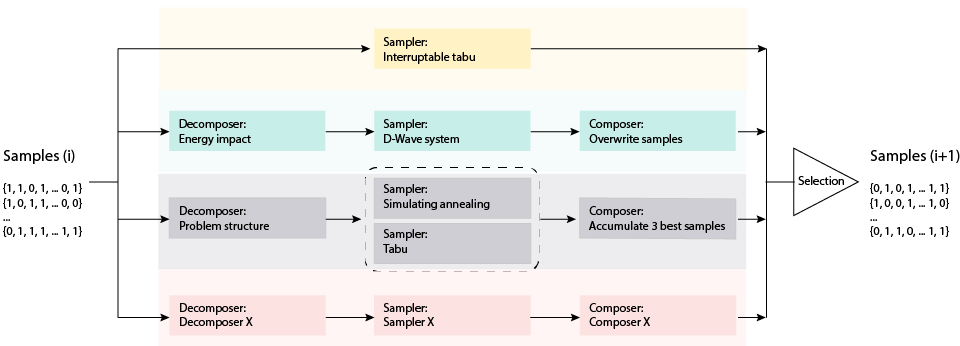
The following Schematic Representation diagram shows an example configuration. The sample iterates over more than four parallel solvers. The top branch represents a classic tabu search that runs on the entire issue until the other branches are interrupted.

These use different resolvers to assign a portion of the current sample set (iteration i) to the sampler, such as D-Wave system (the second highest branch) or other parallel structures such as simulated annealing and tabu search. General representation of branch components (resolver, sampler and combiner), such as the lowest branch. The user-defined criteria are selected from the current sampler and solved to output a sample set for i+1 iterations.

Schematic Representation

You can use the framework to run a supplied hybrid solver or configure workflows using supplied components such as the tabu sampler and the energy based resolver.

You can also use the framework to build your own components to incorporate into workflows.

Using the Framework

This section shows how to use the reference sample to solve problems of any size, and explains how to create (hybrid) workflows using the provided components.

Reference Hybrid Sampler: Kerberos

Dwave hybrid includes a reference sample sampler built using the framework: Kerberos is a dimod compatible hybrid asynchronous decomposition sampler that can solve problems of any structure and size. It finds the best samples by running tabu search, simulated annealing and D-Wave subproblem sampling on the problem variables with high energy influence in parallel.

The following is an example of using Kerberos to solve large QUBO:

import dimod
from hybrid.reference.kerberos import KerberosSampler
with open('../problems/random-chimera/8192.01.qubo') as problem:  
    bqm = dimod.BinaryQuadraticModel.from_coo(problem)
len(bqm)          
8192
solution = KerberosSampler().sample(bqm, max_iter=10, convergence=3)   
solution.first.energy     
-4647.0

Building Workflows

As shown in the Overview section, the hybrid solver is built by arranging components such as samplers in workflows.

Building Blocks

The basic components (Building Blocks) used are based on Runnable classes: resolver, sampler and combiner. This component inputs a set of sample samplesets and outputs the updated samples. The State associated with the components iteration contains problem, sample, and optional additional information.

The following example demonstrates a simple workflow using only one Runnable, which represents the sampler of the classic tabu search algorithm for solving problems (completely classic, without decomposition). This example solves the small problem of triangular graph of nodes with the same coupling. The initial State of all zero samples is used as the starting point set. The solution (new_state) is derived from a single iteration of TabuProblemSampler Runnable.

import dimod
# Define a problem
bqm = dimod.BinaryQuadraticModel.from_ising({}, {'ab': 0.5, 'bc': 0.5, 'ca': 0.5})
# Set up the sampler with an initial state
sampler = TabuProblemSampler(tenure=2, timeout=5)
state = State.from_sample({'a': 0, 'b': 0, 'c': 0}, bqm)
# Sample the problem
new_state = sampler.run(state).result()
print(new_state.samples)                     
    a   b   c  energy  num_occ.
0  +1  -1  -1    -0.5         1
['SPIN', 1 rows, 1 samples, 3 variables]

Flow Structuring

The framework provides for building workflows using "building block" components. As shown in the Overview section, you can create a branch of the Runnable class; For example, decomposer | sampler | composer delegates part of the problem to the sampler, such as the D-Wave system.

The following example shows a decomposer, a local tabu solver, and a composer. A 10 variable quadratic binary model is decomposed into 6-variable subproblems through the energy impact of its variables for two sampling. Use utility function min_sample() sets the initial state of all - 1 values.

import dimod           # Create a binary quadratic model
bqm = dimod.BinaryQuadraticModel({t: 0 for t in range(10)},
                                 {(t, (t+1) % 10): 1 for t in range(10)},
                                 0, 'SPIN')
branch = (EnergyImpactDecomposer(size=6, min_gain=-10) |
          TabuSubproblemSampler(num_reads=2) |
          SplatComposer())
new_state = branch.next(State.from_sample(min_sample(bqm), bqm))
print(new_state.subsamples)      
    4   5   6   7   8   9  energy  num_occ.
0  +1  -1  -1  +1  -1  +1    -5.0         1
1  +1  -1  -1  +1  -1  +1    -5.0         1
['SPIN', 2 rows, 2 samples, 6 variables]

In this way Branch Class can use RacingBranches Run in parallel. From the output of these parallel branches, ArgMin Select a new current sample instead of a single iteration of the sample set, which can be used Loop Iterate the set number of times or until the convergence condition is satisfied.

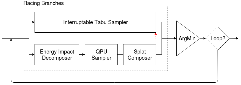
Racing Branches An example is to generate the best samples by iteratively solving a binary quadratic model. and qbsolv Similarly, tabu search is used on the whole problem and D-Wave system is used on the sub problem. In addition to the building block components used above, this example also uses infrastructure classes to manage the decomposition and parallel operation of branches.

Racing Branches

import dimod
import hybrid

# Construct a problem
bqm = dimod.BinaryQuadraticModel({}, {'ab': 1, 'bc': -1, 'ca': 1}, 0, dimod.SPIN)

# Define the workflow
iteration = hybrid.RacingBranches(
    hybrid.InterruptableTabuSampler(),
    hybrid.EnergyImpactDecomposer(size=2)
    | hybrid.QPUSubproblemAutoEmbeddingSampler()
    | hybrid.SplatComposer()
) | hybrid.ArgMin()
workflow = hybrid.LoopUntilNoImprovement(iteration, convergence=3)

# Solve the problem
init_state = hybrid.State.from_problem(bqm)
final_state = workflow.run(init_state).result()

# Print results
print("Solution: sample={.samples.first}".format(final_state))

Flow Refining

The framework can quickly modify workflow to improve solution and performance. For example, validation Racing Branches After branching workflow, some minor problems may need to be modified. For example, the following example can better fit the problem of a large number of variables.

1. Configure a decomposition window to move a small number of problem variables downward, sort from highest to lower energy impact, submit these sub problems to D-Wave system, and conduct global tabu search at the same time. This example submits sub questions of 50 variables, up to 15% of the total variables. This example submits 50 variable until 15% of the total variables.

# Redefine the workflow: a rolling decomposition window
subproblem = hybrid.EnergyImpactDecomposer(size=50, rolling_history=0.15)
subsampler = hybrid.QPUSubproblemAutoEmbeddingSampler() | hybrid.SplatComposer()

iteration = hybrid.RacingBranches(
    hybrid.InterruptableTabuSampler(),
    subproblem | subsampler
) | hybrid.ArgMin()

workflow = hybrid.LoopUntilNoImprovement(iteration, convergence=3)

1. Instead of generating samples in the order of subproblems, further modify and process all subproblems in parallel as much as possible, and then merge the returned samples. EnergyImpactDecomposer Iterate to trigger [endofstream()]( https://docs.ocean.dwavesys.com/en/latest/docs_hybrid/reference/exceptions.html#hybrid.exceptions.EndOfStream )Until it is abnormal (up to 15% of the total variables), and then the sub problem of 50 variable is submitted to the D-Wave system.

# Redefine the workflow: parallel subproblem solving for a single sample
subproblem = hybrid.Unwind(
    hybrid.EnergyImpactDecomposer(size=50, rolling_history=0.15)
)

subsampler = hybrid.Map(
    hybrid.QPUSubproblemAutoEmbeddingSampler()
) | hybrid.Reduce(
    hybrid.Lambda(merge_substates)
) | hybrid.SplatComposer()

1. Change the criteria for selecting subproblems. By default, the selection variable is affected by the maximum energy, but the selection can customize the structure for the problem.

   For example, for Traversal by Energy Impact For the binary quadratic model shown in the illustrated problem graph, if a subproblem of size 4 is selected, these nodes selected by descending energy impact will not be directly connected (there is no shared edge, and may not represent the local structure of the problem).

   

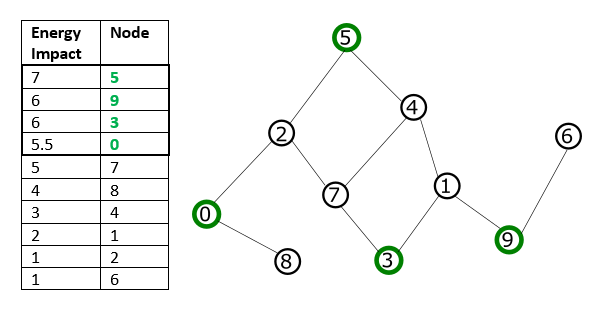
   Traversal by Energy Impact

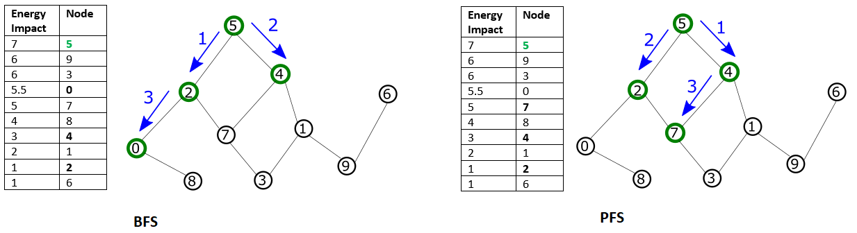
   Configuring traversal patterns such as breadth first (BFS) or priority first selection (PFS) can capture features representing the local structure of the problem.

   # Redefine the workflow: subproblem selection
   subproblem = hybrid.Unwind(
       hybrid.EnergyImpactDecomposer(size=50, rolling_history=0.15, traversal='bfs'))
   

   The graphical forms of the two modes are as follows. BFS starts from the node with the greatest energy impact. From this node, its graph traversal continues to the directly connected nodes, then the nodes directly connected to these nodes, and so on. The graph traversal is sorted by node index. In PFS, graph traversal selects the node with the highest energy impact among the unselected nodes directly connected to any selected node.

   

   Traversal by BFS or PFS

Additional Examples

Tailoring State Selection

The next example customizes a status selector for the sampler, which performs some post-processing and alerts suspicious samples. The output of the sampler modified with ("...") is as follows (Ising model of triangular problem with bias of 0 and interactions of 0.5). The first of the three State classes is marked as problematic:

[{...,'samples': SampleSet(rec.array([([0, 1, 0], 0., 1)], ..., ['a', 'b', 'c'], {'Postprocessor': 'Excessive chain breaks'}, 'SPIN')},
{...,'samples': SampleSet(rec.array([([1, 1, 1], 1.5, 1)], ..., ['a', 'b', 'c'], {}, 'SPIN')},
{...,'samples': SampleSet(rec.array([([0, 0, 0], 0., 1)], ..., ['a', 'b', 'c'], {}, 'SPIN')}]

The following code snippet is in ArgMin Defines the metric of the key parameter.

def preempt(si):
    if 'Postprocessor' in si.samples.info:
        return(math.inf)
    else:
        return(si.samples.first.energy)

Using the key defined above, ArgMin finds the state with the lowest energy state (zero), excluding the marked state (its energy is also zero).

Parallel Sampling

The following code snippet uses Map Tabu search is run in parallel on both States.

Map(TabuProblemSampler()).run(States(                     
        State.from_sample({'a': 0, 'b': 0, 'c': 1}, bqm1),
        State.from_sample({'a': 1, 'b': 1, 'c': 0}, bqm2)))
_.result()                
[{'samples': SampleSet(rec.array([([-1, -1,  1], -0.5, 1)], dtype=[('sample', 'i1', (3,)),
 ('energy', '<f8'), ('num_occurrences', '<i4')]), ['a', 'b', 'c'], {}, 'SPIN'),
 'problem': BinaryQuadraticModel({'a': 0.0, 'b': 0.0, 'c': 0.0}, {('a', 'b'): 0.5, ('b', 'c'): 0.5,
 ('c', 'a'): 0.5}, 0.0, Vartype.SPIN)},
 {'samples': SampleSet(rec.array([([ 1,  1, -1], -1., 1)], dtype=[('sample', 'i1', (3,)),
 ('energy', '<f8'), ('num_occurrences', '<i4')]), ['a', 'b', 'c'], {}, 'SPIN'),
 'problem': BinaryQuadraticModel({'a': 0.0, 'b': 0.0, 'c': 0.0}, {('a', 'b'): 1, ('b', 'c'): 1,
 ('c', 'a'): 1}, 0.0, Vartype.SPIN)}]

Logging and Execution Information

You can view details at the log level.

package supports TRACE, DEBUG, INFO, WARNING, ERROR, and CRITICAL in ascending order of importance. The default level is ERROR. You can use the environment variable DWAVE_HYBRID_LOG_LEVEL to use the log level.

If the environment variable is set to INFO level in Windows OS:

set DWAVE_HYBRID_LOG_LEVEL=INFO

Unix system:

DWAVE_HYBRID_LOG_LEVEL=INFO

The previous example may have the following output:

2018-12-10 15:18:30,634 hybrid.flow INFO Loop Iteration(iterno=0, best_state_quality=-3.0)
2018-12-10 15:18:31,511 hybrid.flow INFO Loop Iteration(iterno=1, best_state_quality=-3.0)
2018-12-10 15:18:35,889 hybrid.flow INFO Loop Iteration(iterno=2, best_state_quality=-3.0)
2018-12-10 15:18:37,377 hybrid.flow INFO Loop Iteration(iterno=3, best_state_quality=-3.0)
Solution: sample=Sample(sample={'a': 1, 'b': -1, 'c': -1}, energy=-3.0, num_occurrences=1)

Developing New Components

*Dwave hybrid * framework can build its own components to add to its own workflow.

The key superclass is the runnable class: all basic components -- samplers, resolvers, composers -- and flow structure components (such as branches) inherit from this class. Runnable runs in an iteration that updates the State it receives. The typical method is run or next to execute the iteration, and stop is to terminate runnable.

Again, Primitives and Flow Structuring This section describes the basic Runnable classes (building blocks) and flow structuring and their methods. If you want to implement these methods for your Runnable class, see the comments in the code.

The following Racing Branches show the top-down component (tree structure) of hybrid loop.

Verify the state of all Runnable objects that inherit from StateTraits or its subclasses. include:

1. minimal check of workflow structure (component of Runnable class);
2. Runtime check;

All built-in Runnable classes declare that state characteristics require independence (for simple ones) or derivation from sub workflows. New Runnable features must be created and modified by the parent class.

Dimod Conversion The HybridRunnable class described in this section can be used to generate a Runnable solver based on the dimod sampler.

Utilities This section provides some useful methods.

Reference Documentation

Some code examples. You can click the link to view it directly.

https://docs.ocean.dwavesys.com/en/latest/docs_hybrid/reference/index.html