Detect DTMF signal quality

Introduction: Using the computer sound card, the telephone sends DTMF signals without connection. Using Python programming, all dial signals are intercepted. The DTMF components are analyzed by FFT and decoded. Experiments show that the control board sends 589 phone numbers without connection, and all the numbers are correct. However, during transmission, it can be seen that there will be an interval for some signals. For example, the following is one of the dialing signals. There is a short time in the middle of the dialing signal.

Key words: DTMF, signal spectrum

§ 00 background

0.1 DTFM telephone dialing standard

DTMF It refers to dual tune multi frequency, which is used for early telephone dial signal transmission. Almost when people begin to use Telegraph and telephone systems to transmit information, people need to find a way to mechanically repeat and reliably interact with the system. Now the signal system can complete these tasks, including wiring, dialing and interacting with the telephone system.
the earliest telephone signal system used was pulse dialing. The following rotary dialing system uses the internal mechanical system to interrupt the telephone connection and generate electrical signals for transmitting telephone dialing information.

▲ Figure 1 telephone with dial dial

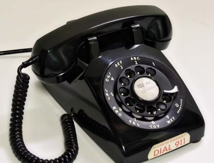
the first dual audio telephone was set in It was first introduced by Bell Laboratories in November 1963 And quickly replaced the rotary dial telephone. The standard used now is ITU Q.23 recommended standards .

▲ Figure 2 Q.23 DTMF model standard

0.2 solving engineering problems

in Interference signal in telephone dual audio dialing sound Medium for Old dialing telephone In the reconstruction project, the Occasional error in telephone dialing . Now pass on Using computer sound card to collect telephone dialing sound Analyze to determine whether the accidental error comes from the internal of the controller system or from the error in connection with the external telephone.

about 3 hours of dialing sound was recorded today (January 21, 2022), which was recorded without a telephone line connected. In this way, it can be judged whether the internal telephone system itself will send some signal faults in the process of sending signals.

Record audio signal: Recording software: Audacity
Recording spectrum: 44.1kHz
Number of channels: 2 (analog signals with the same two channels)
Time: about 3 hours

the telephone number of signal transmission is 18612110728

§ 01 signal analysis

1.1 recording signal

the recorded signal is uploaded to AI Studio and an audio database is established. This data set includes six telephone dual audio signals recorded with a computer sound card.

▲ figure 1.1.1 dual audio telephone number reporting sound

contains signals:

Three offline signals: wav2,sound1,DTFM_RECORD_2022-1-21
Two online signals: ONLINE-WAVE1;ONLINE-WAVE2

1.2 reading and display

1.2.1 wav

(1) Read data

import sys,os,math,time
import matplotlib.pyplot as plt
from numpy import *
from scipy.io import wavfile

filename = '/home/aistudio/data/data126234/wav2.wav'
sample_rate,sig = wavfile.read(filename)
print("sample_rate: {}\n".format(sample_rate), "shape(sig): {}\n".format(shape(sig)))

sample_rate: 44100
shape(sig): (45646080, 2)
sig.shape[0]/sample_rate: 1035.0585034013604

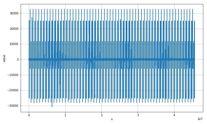
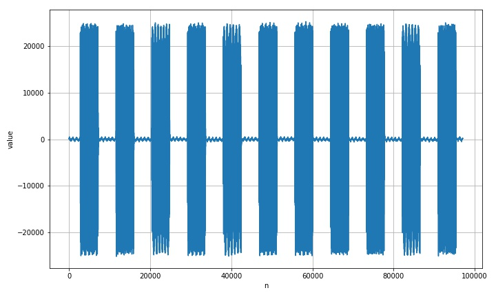
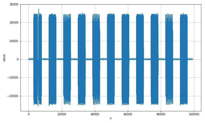
(2) Display signal waveform

plt.clf()
plt.figure(figsize=(10,6))
plt.plot(sig[:,0])
plt.xlabel("n")
plt.ylabel("value")
plt.grid(True)
plt.tight_layout()
plt.savefig('/home/aistudio/stdout.jpg')
plt.show()

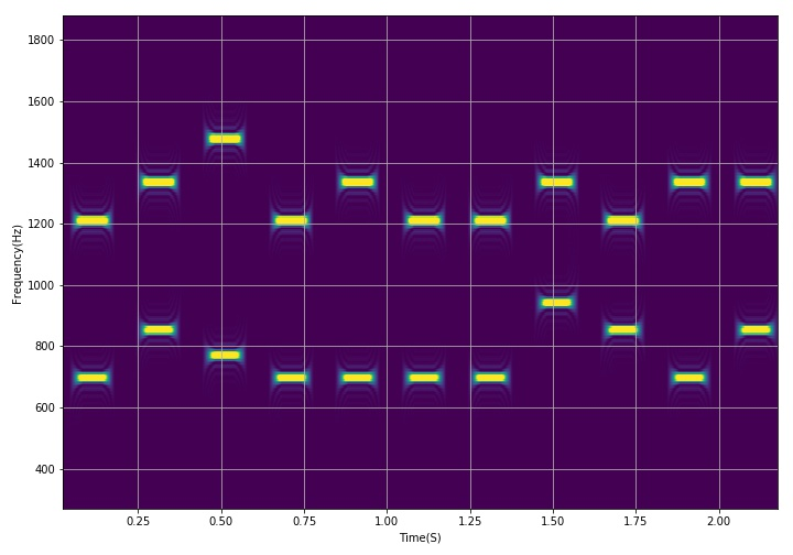
▲ figure 1.2.1 waveforms of all signals

▲ figure 1.2.2 intercepted first dial signal

(3) Video joint distribution of display data

use the signal spectrum function to display the short-time Fourier transform of the data.

▲ short sighted Fourier transform of data

from scipy import signal

f,t,Sxx = signal.spectrogram(sig[startid:endid, 0], fs=sample_rate, nperseg =2048, noverlap=2000, nfft=8192)

thread = 1500000
Sxx[where(Sxx>thread)] = thread

plt.clf()
plt.figure(figsize=(10,7))
plt.pcolormesh(t, f[50:350], Sxx[50:350,:])
plt.xlabel("Time(S)")
plt.ylabel("Frequency(Hz)")
plt.grid(True)
plt.tight_layout()

plt.savefig('/home/aistudio/stdout.jpg')
plt.show()

1.3 effective data interception

in order to judge the data, it is necessary to intercept the effective data first, and then judge whether the spectrum is correct.

1.3.1 basic data parameters

(1) Time interval between two adjacent sets of signals

the following figure shows the waveform relationship between two adjacent dial signals.

▲ two adjacent dialing signals

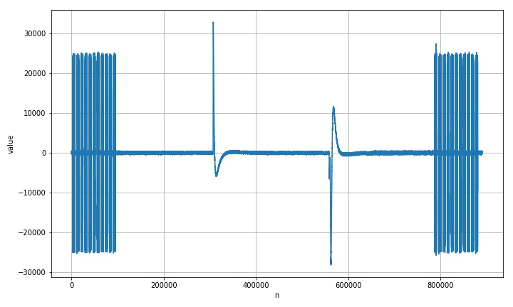
it can be seen from the above waveform that the amplitude of the two high pulse signals generated by the telephone off hook is more than 30000, so the signals can be effectively divided and positioned according to this.

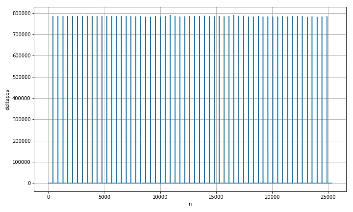
the following is an enlarged image of a sharp pulse waveform.

▲ figure 1.3.2 waveform of a sharp pulse

the position of the pulse can be determined according to the starting position of the rising edge in front of the pulse waveform.

dataseg = list(where(abs(sig[:,0])>0x7f00))
print(dataseg, shape(dataseg))

print(dataseg[:100])

posid = dataseg[0]
posdelta = [s1-s2 for s1,s2 in zip(posid[1:], posid[:-1])]

print(posdelta[:1000])
plt.clf()
plt.figure(figsize=(10,6))
plt.plot(posdelta)
plt.xlabel("n")
plt.ylabel("deltapos")
plt.grid(True)
plt.tight_layout()
plt.savefig('/home/aistudio/stdout.jpg')
plt.show()

[array([  355749,   355750,   355751, ..., 45120329, 45120330, 45120331])]
(1, 25351)
[array([  355749,   355750,   355751, ..., 45120329, 45120330, 45120331])]
[1, 1, 1, 1, 1, 1, 1, 1, 1, 1, 1, 1, 1, 1, 1, 1, 1, 1, 1, 1, 1, 1, 1, 1, 1, 1, 1, 1, 1, 1, 1, 1, 1, 1, 1, 1, 1, 1, 1, 1, 1, 1, 1, 1, 1, 1, 1, 1, 1, 1, 1, 1, 1, 1, 1, 1, 1, 1, 1, 1, 1, 1, 1, 1, 1, 1, 1, 1, 1, 1, 1, 1, 1, 1, 1, 1, 1, 1, 1, 1, 1, 1, 1, 1, 1, 1, 1, 1, 1, 1, 1, 1, 1, 1, 1, 1, 1, 1, 1, 1, 1, 1, 1, 1, 1, 1, 1, 1, 1, 1, 1, 1, 1, 1, 1, 1, 1, 1, 1, 1, 1, 1, 1, 1, 1, 1, 1, 1, 1, 1, 1, 1, 1, 1, 1, 1, 1, 1, 1, 1, 1, 1, 1, 1, 1, 1, 1, 1, 1, 1, 1, 1, 1, 1, 1, 1, 1, 1, 1, 1, 1, 1, 1, 1, 1, 1, 1, 1, 1, 1, 1, 1, 1, 1, 1, 1, 1, 1, 1, 1, 1, 1, 1, 1, 1, 1, 1, 1, 1, 1, 1, 1, 1, 1, 1, 1, 1, 1, 1, 1, 1, 1, 1, 1, 1, 1, 1, 1, 1, 1, 1, 1, 1, 1, 1, 1, 1, 1, 1, 1, 1, 1, 1, 1, 1, 1, 1, 1, 1, 1, 1, 1, 1, 1, 1, 1, 1, 1, 1, 1, 1, 1, 1, 1, 1, 1, 1, 1, 1, 1, 1, 1, 1, 1, 1, 1, 1, 1, 1, 1, 1, 1, 1, 1, 1, 1, 1, 1, 1, 1, 1, 1, 1, 1, 1, 1, 1, 1, 1, 1, 1, 1, 1, 1, 1, 1, 1, 1, 1, 1, 1, 1, 1, 1, 1, 1, 1, 1, 1, 1, 1, 1, 1, 1, 1, 1, 1, 1, 1, 1, 1, 1, 1, 1, 1, 1, 1, 1, 1, 1, 1, 1, 1, 1, 1, 1, 1, 1, 1, 1, 1, 1, 1, 1, 1, 1, 1, 1, 1, 1, 1, 1, 1, 1, 1, 1, 1, 1, 1, 1, 1, 1, 1, 1, 1, 1, 1, 1, 1, 1, 1, 1, 1, 1, 1, 1, 1, 1, 1, 1, 1, 1, 1, 1, 1, 1, 1, 1, 1, 1, 1, 1, 1, 1, 1, 1, 1, 1, 1, 1, 1, 1, 1, 1, 1, 1, 1, 1, 1, 1, 1, 1, 1, 1, 1, 1, 1, 1, 1, 1, 1, 1, 1, 1, 1, 1, 1, 1, 1, 1, 1, 1, 1, 1, 1, 1, 1, 1, 1, 1, 1, 1, 1, 1, 786481, 1, 1, 1, 1, 1, 1, 1, 1, 1, 1, 1, 1, 1, 1, 1, 1, 1, 1, 1, 1, 1, 1, 1, 1, 1, 1, 1, 1, 1, 1, 1, 1, 1, 1, 1, 1, 1, 1, 1, 1, 1, 1, 1, 1, 1, 1, 1, 1, 1, 1, 1, 1, 1, 1, 1, 1, 1, 1, 1, 1, 1, 1, 1, 1, 1, 1, 1, 1, 1, 1, 1, 1, 1, 1, 1, 1, 1, 1, 1, 1, 1, 1, 1, 1, 1, 1, 1, 1, 1, 1, 1, 1, 1, 1, 1, 1, 1, 1, 1, 1, 1, 1, 1, 1, 1, 1, 1, 1, 1, 1, 1, 1, 1, 1, 1, 1, 1, 1, 1, 1, 1, 1, 1, 1, 1, 1, 1, 1, 1, 1, 1, 1, 1, 1, 1, 1, 1, 1, 1, 1, 1, 1, 1, 1, 1, 1, 1, 1, 1, 1, 1, 1, 1, 1, 1, 1, 1, 1, 1, 1, 1, 1, 1, 1, 1, 1, 1, 1, 1, 1, 1, 1, 1, 1, 1, 1, 1, 1, 1, 1, 1, 1, 1, 1, 1, 1, 1, 1, 1, 1, 1, 1, 1, 1, 1, 1, 1, 1, 1, 1, 1, 1, 1, 1, 1, 1, 1, 1, 1, 1, 1, 1, 1, 1, 1, 1, 1, 1, 1, 1, 1, 1, 1, 1, 1, 1, 1, 1, 1, 1, 1, 1, 1, 1, 1, 1, 1, 1, 1, 1, 1, 1, 1, 1, 1, 1, 1, 1, 1, 1, 1, 1, 1, 1, 1, 1, 1, 1, 1, 1, 1, 1, 1, 1, 1, 1, 1, 1, 1, 1, 1, 1, 1, 1, 1, 1, 1, 1, 1, 1, 1, 1, 1, 1, 1, 1, 1, 1, 1, 1, 1, 1, 1, 1, 1, 1, 1, 1, 1, 1, 1, 1, 1, 1, 1, 1, 1, 1, 1, 1, 1, 1, 1, 1, 1, 1, 1, 1, 1, 1, 1, 1, 1, 1, 1, 1, 1, 1, 1, 1, 1, 1, 1, 1, 1, 1, 1, 1, 1, 1, 1, 1, 1, 1, 1, 1, 1, 1, 1, 1, 1, 1, 1, 1, 1, 1, 1, 1, 1, 1, 1, 1, 1, 1, 1, 1, 1, 1, 1, 1, 1, 1, 1, 1, 1, 1, 1, 1, 1, 1, 1, 1, 1, 1, 1, 1, 1, 1, 1, 1, 1, 1, 1, 1, 1, 1, 1, 1, 1, 1, 1, 1, 1, 1, 1, 1, 1, 1, 1, 1, 1, 1, 1, 1, 1, 1, 1, 1, 1, 1, 1, 1, 1, 1, 1, 1, 1, 1, 1, 1, 1, 1, 1, 1, 1, 4, 1, 1, 1, 1, 1, 785271, 1, 1, 1, 1, 1, 1, 1, 1, 1, 1, 1, 1, 1, 1, 1, 1, 1, 1, 1, 1, 1, 1, 1, 1, 1, 1, 1, 1, 1, 1, 1, 1, 1, 1, 1, 1, 1, 1, 1, 1, 1, 1, 1, 1, 1, 1, 1, 1, 1, 1, 1, 1, 1, 1, 1, 1, 1, 1, 1, 1, 1, 1, 1, 1, 1, 1, 1, 1, 1, 1, 1, 1, 1, 1, 1, 1, 1, 1, 1, 1, 1, 1, 1, 1, 1, 1, 1, 1, 1, 1, 1, 1, 1, 1, 1, 1, 1, 1, 1, 1, 1, 1, 1, 1, 1, 1, 1, 1, 1, 1, 1, 1, 1, 1, 1, 1, 1, 1, 1, 1, 1, 1, 1]

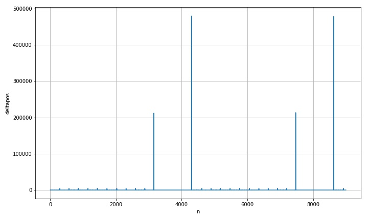
▲ figure 1.3.3 waveforms corresponding to all rising edges

the interval between these rising pulses is:

pd = array(posdelta)
possplit = pd[where(pd > 1000)]
print("possplit: {}\n".format(possplit), "len(possplit): {}\n".format(len(possplit)), "mean(possplit): {}\n".format(mean(possplit)), "mean(possplit)/sample_rate: {}\n".format(mean(possplit)/sample_rate))

possplit: [786481 785271 786005 785485 785631 785996 785302 786970 785405 784943
 786674 784894 785761 785753 786155 784973 786987 783855 784476 783570
 782555 784458 782916 785667 789454 784251 783545 783764 784366 784989
 784486 787431 784040 783745 785528 783743 784939 789109 785727 787110
 783177 783532 786536 783833 784088 783743 783043 783922 782797 784285
 784523 784822 782861 784441 783300 783629 784274]

len(possplit): 57
mean(possplit): 784898.5263157894
mean(possplit)/sample_rate: 17.798152524167563

from the above results, there are 57 dialing segments in wav2file, and the average time interval between them is: T s = 17.8 s T_s = 17.8s Ts=17.8s

1.3.2 data interception

intercepted data refers to the audio data intercepted by dialing 11 pulses.

▲ figure 1.3.4 signal waveform

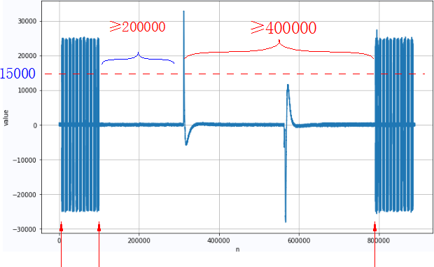
the corresponding time interval before the dial signal is greater than 400000.

wavefilename = '/home/aistudio/data/data126234/wav2.wav'

sample_rate,sig = wavfile.read(wavefilename)

dataseg = list(where(sig[:,0] > 20000))
posid = dataseg[0]
posdelta = [s1-s2 for s1,s2 in zip(posid[1:], posid[:-1])]

plt.clf()
plt.figure(figsize=(10,6))
plt.plot(posdelta[:9000], label='POSDELTA')
plt.xlabel("n")
plt.ylabel("deltapos")
plt.grid(True)
plt.tight_layout()
plt.savefig('/home/aistudio/stdout.jpg')
plt.show()

▲ figure 1.3.5 first two segments of data

the starting position of telephone signal is given below.

beginid = array(list(zip(posid[1:],posid[:-1])))[where(posdelta > 400000)]
print("beginid.T: {}\n".format(beginid.T), "shape(beginid): {}\n".format(shape(beginid)))

beginid.T: [[  836306  1621745  2408903  3193945  3980233  4765672  5551524  6339190
   7124987  7912553  8698676  9484556 10269399 11054722 11842377 12629740
  13414451 14203456 14986067 15770299 16553373 17339407 18122751 18908758
  19698392 20481857 21268481 22049985 22836030 23620779 24406880 25192396
  25979819 26763351 27549539 28332773 29118796 29908430 30692265 31480796
  32266869 33047810 33835365 34619228 35405796 36189780 36973047 37755785
  38542178 39324767 40108260 40895783 41678995 42463568 43246945 44032197
  44816043 45602380]
 [  356796  1143719  1929410  2715871  3501790  4287880  5074302  5860021
   6647411  7433280  8218650  9005777  9791085 10577298 11363487 12150076
  12935483 13722878 14507173 15292070 16076090 16859083 17643994 18427354
  19213444 20003346 20788030 21572011 22356204 23141016 23926446 24711360
  25499256 26283716 27067917 27853868 28638069 29423430 30212969 30999135
  31786684 32570306 33354257 34141237 34925519 35710046 36494197 37277688
  38062044 38845293 39630016 40414985 41200222 41983539 42768398 43552158
  44336209 45120939]]

shape(beginid): (58, 2)

(1) Intercept a piece of data

wavetime = 2.25
wavelength = int(sample_rate * wavetime)

startid = beginid.T[0][0] - 3000
endid = startid + wavelength

plt.clf()
plt.figure(figsize=(10,6))
plt.plot(sig[startid:endid, 0])
plt.xlabel("n")
plt.ylabel("value")
plt.grid(True)
plt.tight_layout()
plt.savefig('/home/aistudio/stdout.jpg')
plt.show()

▲ figure 1.3.6 intercepting a section of data

there are 58 starting points in front, but the length of the last waveform is not enough for a complete dialing limit. Next, the first 57 groups of dialing signals will be intercepted.

▲ there are 57 waveforms intercepted in the figure

corresponding to the joint distribution of video obtained by short-time Fourier transform.

▲ short time Fourier transform of the data intercepted in Fig

gifpath = '/home/aistudio/GIF'
if not os.path.isdir(gifpath):
    os.makedirs(gifpath)
gifdim = os.listdir(gifpath)
for f in gifdim:
    fn = os.path.join(gifpath, f)
    if os.path.isfile(fn):
        os.remove(fn)

count = 0
for id in tqdm(beginid.T[0][:-1]):
    startid = id - 3000
    endid = startid + wavelength

    f,t,Sxx = signal.spectrogram(sig[startid:endid, 0], fs=sample_rate,
                            nperseg =2048, noverlap=2000, nfft=8192)

    thread = 1500000
    Sxx[where(Sxx>thread)] = thread

    plt.clf()
    plt.figure(figsize=(10,6))
    plt.pcolormesh(t, f[50:350], Sxx[50:350,:])
    plt.xlabel("Time(S)")
    plt.ylabel("Frequency(Hz)")
    plt.grid(True)
    plt.tight_layout()
    savefile = os.path.join(gifpath, '%03d.jpg'%count)
    count += 1
    plt.savefig(savefile)

1.4 judgment data telephone number

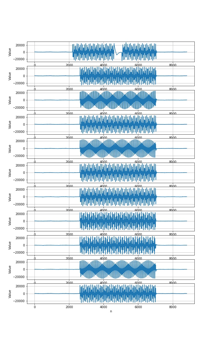
1.4.1 divide the dial signal into 11 equal parts

wavetime = 2.2
wavelength = int(sample_rate * wavetime)

startid = beginid.T[0][0] - 2200
endid = startid + wavelength

segpos = [int(s) for s in linspace(startid, endid, 12, endpoint=True)]

plt.clf()
plt.figure(figsize=(10,16))

for i in range(11):
    plt.subplot(11,1,i+1)
    plt.plot(sig[segpos[i]:segpos[i+1], 0])
    plt.xlabel('n')
    plt.ylabel('Value')
    plt.grid(True)

plt.savefig('/home/aistudio/stdout.jpg')
plt.show()

▲ figure 1.4.1 divides the telephone number signal into 11 equal parts

1.4.2 judge the coding of a section of signal

(1) Calculate the FFT of the signal

calculate the spectrum of the signal through FFT. The spectrum between 500 and 1800hz is shown below.

segnum = sig[segpos[0]:segpos[1], 0]
fftabs = abs(fft.fft(segnum))/len(segnum)

fstart = 500
fend = 1800
fmid = 1075
fstartid = int(len(segnum)*fstart/sample_rate)
fendid = int(len(segnum)*fend/sample_rate)

fdim = linspace(0, sample_rate, len(segnum))

plt.clf()
plt.figure(figsize=(10,6))
plt.plot(fdim[fstartid:fendid], fftabs[fstartid:fendid])
plt.xlabel("Frequency")
plt.ylabel("Amplitude")
plt.grid(True)
plt.tight_layout()
plt.savefig('/home/aistudio/stdout.jpg')
plt.show()

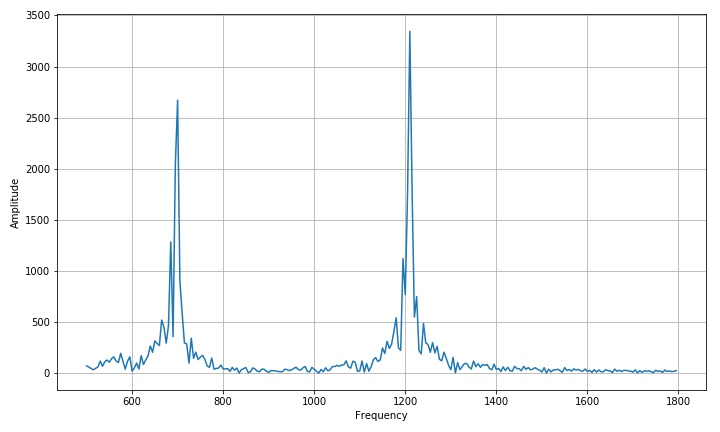
▲ figure 1.4.2 FFT amplitude spectrum of signal

(2) Calculate low frequency and high frequency peaks

search the frequency corresponding to the peak at (500 ~ 1075) and (10751800) respectively.

lowfft = fftabs[fstartid:fmidid]
highfft = fftabs[fmidid:fendid]

lowid = where(lowfft==max(lowfft))[0][0]+fstartid
highid = where(highfft==max(highfft))[0][0]+fmidid
lowf = lowid * sample_rate/len(segnum)
highf = highid * sample_rate/len(segnum)
print("lowf: {}\n".format(lowf), "highf: {}\n".format(highf))

lowf: 700.0

highf: 1210.0

(3) Judge corresponding code

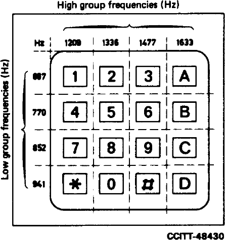
according to DTMF The low frequency and high frequency coding scheme of DTMF is given. Judge the corresponding code according to lowf and HIGHF.

lowfdim = [697, 770, 852, 941]
highfdim = [1209, 1336, 1477, 1633]
deltaf = 25

def freq2code(lowf, highf):
    lowid = 0
    highid = 0

    for i,f in enumerate(lowfdim):
        if lowf >= f-deltaf and lowf < f+deltaf:
            lowid = i
            break

    for i,f in enumerate(highfdim):
        if highf >= f-deltaf and highf < f+deltaf:
            highid = i
            break

    idid = lowid + highid*4

    return "147*2580369#ABCD"[idid]

 '''
code = freq2code(lowf, highf)
print("code: {}\n".format(code))
 '''
def wave2phone(wavedata, fs):
    segpos = [int(s) for s in linspace(0, len(wavedata), 12, endpoint=True)]

    fstart = 500
    fend = 1800
    fmid = 1075
    code = ''
    for i in range(11):
        wave = wavedata[segpos[i]:segpos[i+1]]

        fstartid = int(len(wave)*fstart/fs)
        fendid = int(len(wave)*fend/fs)
        fmidid = int(len(wave)*fmid/fs)

        fftabs = abs(fft.fft(wave))/len(wave)
        lowfft = fftabs[fstartid:fmidid]
        highfft = fftabs[fmidid:fendid]

        lowid = where(lowfft==max(lowfft))[0][0]+fstartid
        highid = where(highfft==max(highfft))[0][0]+fmidid
        lowf = lowid * fs /len(wave)
        highf = highid * fs /len(wave)

        code = code + freq2code(lowf, highf)

    return code

wavetime = 2.2
wavelength = int(sample_rate * wavetime)
startid = beginid.T[0][0] - 2200
endid = startid + wavelength
ret = wave2phone(sig[startid:endid, 0], sample_rate)

print("ret: {}\n".format(ret))

the decoded output is as follows. It can be seen that it is consistent with the transmitted data.
ret: 18612110728

1.5 process all dial signals

wavetime = 2.2
wavelength = int(sample_rate * wavetime)

for ii in beginid.T[0][:-1]:
    startid = ii - 2200
    endid = startid + wavelength
    ret = wave2phone(sig[startid:endid, 0], sample_rate)
    print("ret: {}\n".format(ret))

the 57 dialing codes obtained are the same.

ret: 18612110728
ret: 18612110728
ret: 18612110728
ret: 18612110728
.......
ret: 18612110728
ret: 18612110728
ret: 18612110728
ret: 18612110728
ret: 18612110728

§ 02 processing data

according to the algorithm given above, the received dialing data is processed below.

2.1 processing complete code

from headm import *                 # =

from scipy                  import signal
from scipy.io               import wavfile
from tqdm import tqdm

wavefilename = '/home/aistudio/data/data126234/wav2.wav'

sample_rate,sig = wavfile.read(wavefilename)

dataseg = list(where(sig[:,0] > 20000))
posid = dataseg[0]
beginid = array(list(zip(posid[1:],posid[:-1])))[where(posdelta > 400000)]

lowfdim = [697, 770, 852, 941]
highfdim = [1209, 1336, 1477, 1633]
deltaf = 25

def freq2code(lowf, highf):
    lowid = 0
    highid = 0

    for i,f in enumerate(lowfdim):
        if lowf >= f-deltaf and lowf < f+deltaf:
            lowid = i
            break

    for i,f in enumerate(highfdim):
        if highf >= f-deltaf and highf < f+deltaf:
            highid = i
            break

    idid = lowid + highid*4

    return "147*2580369#ABCD"[idid]

def wave2phone(wavedata, fs):
    segpos = [int(s) for s in linspace(0, len(wavedata), 12, endpoint=True)]

    fstart = 500
    fend = 1800
    fmid = 1075
    code = ''
    for i in range(11):
        wave = wavedata[segpos[i]:segpos[i+1]]

        fstartid = int(len(wave)*fstart/fs)
        fendid = int(len(wave)*fend/fs)
        fmidid = int(len(wave)*fmid/fs)

        fftabs = abs(fft.fft(wave))/len(wave)
        lowfft = fftabs[fstartid:fmidid]
        highfft = fftabs[fmidid:fendid]

        lowid = where(lowfft==max(lowfft))[0][0]+fstartid
        highid = where(highfft==max(highfft))[0][0]+fmidid
        lowf = lowid * fs /len(wave)
        highf = highid * fs /len(wave)

        code = code + freq2code(lowf, highf)

    return code

wavetime = 2.2
wavelength = int(sample_rate * wavetime)

error = 0
for ii in beginid.T[0][:-1]:
    startid = ii - 2200
    endid = startid + wavelength
    ret = wave2phone(sig[startid:endid, 0], sample_rate)
    if ret != '18612110728': error += 1

printt(len(beginid.T[0])-1:, error:)

2.1.1 processing two wave files

(1) wav processing results

output result:

len(beginid.T[0])-1: 57	
error: 0

(2) wav processing results

len(beginid.T[0])-1: 22
error: 0

2.1.2 processing and recording MP3 files

recorded DTMF-RECORD_2022-1-21.mp3, recording 10511 seconds of sound.

(1) Documents

wavefilename = '/home/aistudio/data/data126234/DTFM-RECORD-2022-1-21.mp3'

sound = AudioSegment.from_file(file=wavefilename)
left = sound.split_to_mono()[0]
sample_rate = sound.frame_rate
sig = frombuffer(left._data, int16)

the total data is 463552000 sampling data. Due to the large amount of data, you need to use the supreme configuration of 32G memory in AI Studio to process this data. In the normal version of the configuration, the system always crashes.

(2) Processing results

after 56.8 seconds of operation, the processing results are as follows:

sample_rate: 44100
len(beginid.T[0])-1: 589
error: 0

a total of 589 telephone dialing codes, and the transmitted output is correct.

※ test summary ※

the voice card of the computer is used to record the DTMF signal sent by the telephone without connection. All dial signals are intercepted by Python programming. The DTMF components are analyzed by FFT and decoded. Experiments show that the control board sends 589 phone numbers without connection, and all the numbers are correct.

however, during transmission, it can be seen that there will be intervals for some signals. For example, the following is one of the dialing signals. There is a short time in the middle of the dialing signal.

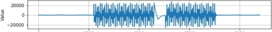
▲ Figure 3.1 there is an interval between transmitted signals

in principle, if the intermediate break is judged to be two dialing signals, it will cause telephone number error. Therefore, it is necessary to make a statistical judgment on this situation. Is this middle section common? How long will the break be?

■ links to relevant literature:

● links to relevant charts:

Figure 1 telephone with dial dial
Figure 2 Q.23 DTMF model standard
Figure 1.1.1 dual audio telephone number reporting sound
Figure 1.2.1 waveforms of all signals
Figure 1.2.2 intercepted first dial signal
Short sighted Fourier transform of data
Adjacent two dialing signals
Figure 1.3.2 waveform of a sharp pulse
Figure 1.3.3 waveforms corresponding to all rising edges
Figure 1.3.4 signal waveform
Figure 1.3.5 first two segments of data
Figure 1.3.6 intercepting a section of data
Fig. 57 waveforms are intercepted
Fig. short time Fourier transform of intercepted data
Figure 1.4.1 dividing the telephone number signal into 11 equal parts
Fig. 1.4.2 FFT amplitude spectrum of signal
Figure 3.1 interval between transmitted signals

Added by digitalbart2k on Sat, 22 Jan 2022 00:53:39 +0200

Programming VIP