1, Brief introduction of digital baseband signal waveform simulation

This paper mainly studies the basic concept of digital signal baseband transmission, the transmission process of digital signal baseband transmission, and how to simulate and design digital baseband transmission system with MATLAB software. Firstly, this paper introduces the MATLAB simulation software. Then it introduces the theoretical basis of this subject, including digital communication, the composition of digital baseband transmission system and the transmission process of digital baseband signal. Then it introduces the characteristics of digital baseband transmission system, including digital PAM signal power density and common line code types, and finally selects bipolar non return to zero code by comparison. Then it introduces the best receiving conditions of digital baseband signal and how to observe the waveform of baseband signal through oscilloscope. Finally, according to the basic steps of the simulation process, the simulation process of the digital baseband transmission system is realized with the simulation tool of MATLAB, and the system is analyzed.

Although the application of digital baseband transmission system in actual digital communication system is not as wide as band transmission, it still has a considerable range of applications. And most importantly, the basic theory of digital baseband transmission system is not only applicable to digital baseband transmission system, but also applicable to frequency band transmission, because all narrow band-pass signals, linear band-pass systems and equivalent low-pass systems can use their equivalent low-pass signals The equivalent low-pass system and the response of the equivalent low-pass system to the equivalent low-pass signal, so the band transmission system can study its performance through the theoretical analysis and computer simulation of its equivalent low-pass (or equivalent baseband) transmission system. Therefore, it is very important to master the basic theory of digital baseband transmission, which is of universal significance in digital communication system.

1 Introduction to baseband transmission system
If the carrier of the digital modulator is a periodic pulse, the digital sequence can be converted into the corresponding signal waveform by modulating a certain parameter of the pulse carrier with the digital sequence, which is called the digital pulse modulator. The power spectral density of the output signal waveform of the digital pulse modulator is low-pass, the occupied frequency band starts from DC or low frequency, and its bandwidth is limited. Then this digital signal is called digital baseband signal. If the transfer function of the communication channel is low-pass, the channel is called baseband channel, which is also called low-pass channel, just as the shaft cable and twisted pair cable channel belong to baseband channel. Digital baseband signal is transmitted through baseband channel, so this transmission system is called digital baseband transmission system.

2. Structure diagram of baseband transmission system

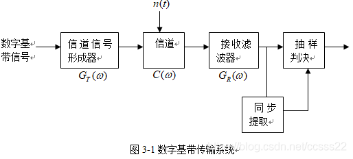
The baseband transmission system is mainly composed of channel signal generator, channel, receiving filter and sampling decision maker. In order to ensure the reliable and orderly operation of the system, there should also be a synchronization system.
Channel signal former: transforms the original baseband signal into a baseband signal suitable for channel transmission. This transformation is mainly realized through code type transformation and waveform transformation. Its purpose is to match with the channel, facilitate transmission, reduce inter symbol crosstalk, and facilitate synchronous extraction and sampling decision.
Channel: a medium that allows baseband signals to pass through. The transmission characteristics of the channel usually do not meet the distortion free transmission conditions, or even change randomly. In addition, the channel will enter noise. In the analysis of communication system, noise n (t) is often equivalent and introduced into the channel.
Receiving filter: filter out of band noise and equalize channel characteristics, so that the output baseband waveform is conducive to sampling decision.
Sample decider: under the background of unsatisfactory transmission characteristics and noise, sample and judge the output waveform of the receiving filter at a specified time (controlled by bit timing pulse) to recover or regenerate the baseband signal. The bit timing pulse used for sampling is extracted from the received signal by the synchronous extraction circuit. The accuracy of bit timing will directly affect the decision effect.

3 baseband transmission process

The pulse sequence generated by the encoder of the terminal equipment will be used as the input signal of the baseband transmission system. In order to enable this pulse sequence to be transmitted in the channel, it is generally necessary to change the binary pulse sequence into bipolar code (AMI code or HDB3 code) through the code converter. Sometimes, in order to minimize the inter symbol interference of the signal in the baseband transmission system, waveform conversion is also required. Because the channel characteristics are not ideal or the interference of noise, the signal passing through the channel will be disturbed and deformed. At the receiving end, in order to reduce the influence of noise, the signal passing through the channel will first be introduced into the receiving filter, and then pass through the equalizer to correct the waveform distortion or inter symbol crosstalk caused by the unsatisfactory channel characteristics (including the receiving filter). Finally, when the sampling timing pulse arrives, a decision is made to recover the baseband digital code pulse.

2, Partial source code

close all
clear all
%Setting of sampling points
k=14;
%Setting of samples per symbol
L= 32;
N=2^k;
M=N/L;%M Is the number of symbols
dt=1/L;%Time domain sampling interval
T=N*dt;%Time domain truncation interval
df=1.0/T;%Frequency domain sampling interval
Bs=N*df/2;%Frequency domain truncation interval
t=linspace(-T/2,T/2,N);%Generate time domain sampling points
f=linspace(-Bs,Bs,N);%Generate frequency domain sampling points
EP1=zeros(size(f));
EP2=zeros(size(f));
EP3=zeros(size(f));

%Program part 1: randomly generate 1000 columns of 0 and 1 signal sequences, and perform bipolar zeroing coding and non zeroing respectively%Code, and calculate their respective power spectral density and the mean value of power spectral density
for x=1:1000%Take 1000 samples
    a=round(rand(1,M));%Generate a length of M Random sequence of a，0 And 1
    nrz=zeros(L,M);%Generate a L that 's ok M Columnar nrz Matrix, initialized to all 0 matrix
    rz=zeros(L,M);%Generate a L that 's ok M Columnar rz Matrix, initialized to all 0 matrix
    for i=1:M 
        if a(i)==1
            nrz(:,i)=1;%send nrz Matrix No i All elements of the column are 1
            rz(1:L/2,i)=1;%send rz Matrix No i Before column L/2 1 element
        else
            nrz(:,i)=0;%send nrz Matrix No i All elements of the column are-1
            rz(1:L/2,i)=0;%send rz Matrix No i Before column L/2 Elements are-1
        end
    end    
    %Rearrange separately nrz,rz The matrix is 1 row N Matrix of columns
    nrz=reshape(nrz,1,N);
    rz=reshape(rz,1,N);
    %Do Fourier transform and calculate the power spectral density
    NRZ=t2f(nrz,dt);
    P1=NRZ.*conj(NRZ)/T;
    RZ=t2f(rz,dt);
    P2=RZ.*conj(RZ)/T;
    %Find the mean of power spectral density
    EP1=(EP1*(x-1)+P1)/x;
    EP2=(EP2*(x-1)+P2)/x;
end
%Setting of sampling points
k=14;
%Setting of samples per symbol
L= 32;
N=2^k;
M=N/L;%M Is the number of symbols
dt=1/L;%Time domain sampling interval
T=N*dt;%Time domain truncation interval
df=1.0/T;%Frequency domain sampling interval
Bs=N*df/2;%Frequency domain truncation interval
t=linspace(-T/2,T/2,N);%Generate time domain sampling points
f=linspace(-Bs,Bs,N);%Generate frequency domain sampling points
EP1=zeros(size(f));
EP2=zeros(size(f));
EP3=zeros(size(f));

%Part 2 of the program: randomly generate 1000 columns of 0 and 1 signal sequences, and carry out bipolar zeroing coding and non zeroing respectively%Code, and calculate their respective power spectral density and the mean value of power spectral density
for x=1:1000%Take 1000 samples
    a=round(rand(1,M));%Generate a length of M Random sequence of a，0 And 1
    nrz=zeros(L,M);%Generate a L that 's ok M Columnar nrz Matrix, initialized to all 0 matrix
    rz=zeros(L,M);%Generate a L that 's ok M Columnar rz Matrix, initialized to all 0 matrix
    for i=1:M 
        if a(i)==1
            nrz(:,i)=1;%send nrz Matrix No i All elements of the column are 1
            rz(1:L/2,i)=1;%send rz Matrix No i Before column L/2 1 element
        else
            nrz(:,i)=-1;%send nrz Matrix No i All elements of the column are-1
            rz(1:L/2,i)=-1;%send rz Matrix No i Before column L/2 Elements are-1
        end
    end
    
    %Rearrange separately nrz,rz The matrix is 1 row N Matrix of columns
    nrz=reshape(nrz,1,N);
    rz=reshape(rz,1,N);
    %Do Fourier transform and calculate the power spectral density
    NRZ=t2f(nrz,dt);
    P1=NRZ.*conj(NRZ)/T;
    RZ=t2f(rz,dt);
    P2=RZ.*conj(RZ)/T;
    %Find the mean of power spectral density
    EP1=(EP1*(x-1)+P1)/x;
    EP2=(EP2*(x-1)+P2)/x;
end

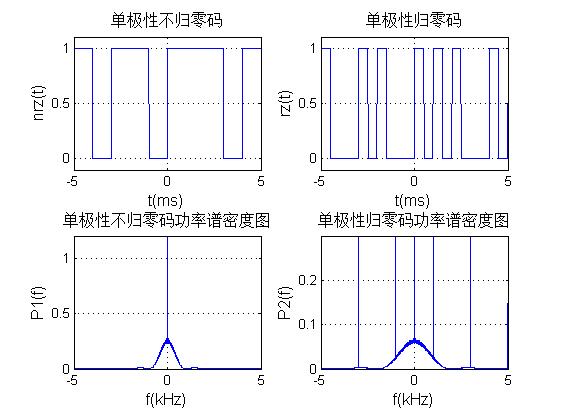
3, Operation results

4, matlab version and references

1 matlab version
2014a

2 references
[1] Shen Zaiyang. Proficient in MATLAB signal processing [M]. Tsinghua University Press, 2015
[2] Gao Baojian, Peng Jinye, Wang Lin, pan Jianshou. Signal and system -- Analysis and implementation using MATLAB [M]. Tsinghua University Press, 2020
[3] Wang Wenguang, Wei Shaoming, Ren Xin. MATLAB implementation of signal processing and system analysis [M]. Electronic Industry Press, 2018