In the time domain, the method to describe the characteristics of the system is the difference equation and the unit impulse response.
In the frequency domain, the method of describing the characteristics of the system can be the system function
Linear time invariant property of system, causality, stability
Stability is that the system can obtain a bounded response to any bounded input signal.
The unit impulse response of the system satisfies absolute summability
The stability of the system can be obtained from the coefficients of the difference equation
The most common way to check the system stability is to input the unit step sequence. When n →∞, the system output approaches a constant, then the system is stable

Example 1

Given a difference equation
y(n)=0.05x(n)+0.05x(n-1)+0.9y(n-1)
Input signal x(n)=R8(n)
Find the system response of x(n) and draw the waveform
Find the unit impulse response

clc
close all;
clear all;
A=[1,-0.9];
B=[0.05,0.05];
xn=[ones(1,8),zeros(1,42)];
n=0:length(xn)-1;
[hn,n]=impz(B,A,length(xn));
yn=filter(B,A,xn);
figure
subplot(2,1,1);
xlabel('n');
ylabel('y(n)');
stem(n,yn,'.');
axis([0,length(n),min(yn),1.2*max(yn)]);
title('System response to R8(n)');

subplot(2,1,2);
xlabel('n');
ylabel('h(n)');
stem(n,hn,'.');
axis([0,length(n),min(hn),1.2*max(hn)]);
title('System unit impulse response');

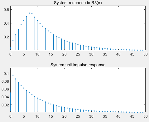
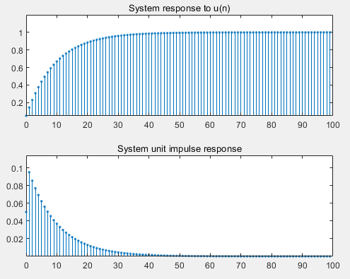
The signal passes through the low-pass filter, the high frequency of the signal is filtered, the change of the time-domain signal slows down, and a transition band is generated near the step. Therefore, when the rectangular sequence is input, there is an obvious transition zone at the beginning and end of the output sequence. When the input is a unit step, an obvious transition zone is also generated

Example 2

Given a difference equation
y(n)=0.05x(n)+0.05x(n-1)+0.9y(n-1)
Input signal x(n)=u(n)
Find the system response of x(n) and draw the waveform
Find the unit impulse response

clc
close all;
clear all;
A=[1,-0.9];
B=[0.05,0.05];
xn=ones(1,100);
n=0:length(xn)-1;
[hn,n]=impz(B,A,length(xn));
yn=filter(B,A,xn);
figure
subplot(2,1,1);
xlabel('n');
ylabel('y(n)');
stem(n,yn,'.');
axis([0,length(n),min(yn),1.2*max(yn)]);
title('System response to u(n)');

subplot(2,1,2);
xlabel('n');
ylabel('h(n)');
stem(n,hn,'.');
axis([0,length(n),min(hn),1.2*max(hn)]);
title('System unit impulse response');

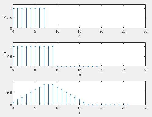
Example 3

Unit impulse response of a given system h(n)=R10(n),
The output response y(n) of x(n)=R8(n) to system h(n) is obtained by linear convolution method

clc
close all;
clear all;
xn=ones(1,8);
n=0:length(xn)-1;
figure
subplot(3,1,1);
stem(n,xn,'.');
xlabel('n');
ylabel('xn');
axis([0,30,0,1.2*max(xn)]);

hn=[ones(1,10),zeros(1,10)];
m=0:length(hn)-1;
subplot(3,1,2);
stem(m,hn,'.');
xlabel('m');
ylabel('hn');
axis([0,30,0,1.2*max(hn)]);

yn=conv(hn,xn)
l=0:length(xn)+length(hn)-2;
subplot(3,1,3);
stem(l,yn,'.');
xlabel('l');
ylabel('yn');
axis([0,30,0,1.2*max(yn)]);

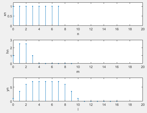
Example 4

Unit impulse response h(n) of a given system= δ (n)+2.5 δ (n-1)+2.5 δ (n-2)+ δ (n-3)
The output response y(n) of x(n)=R8(n) to system h(n) is obtained by linear convolution method

clc
close all;
clear all;
xn=ones(1,8);
n=0:length(xn)-1;
figure
subplot(3,1,1);
stem(n,xn,'.');
xlabel('n');
ylabel('xn');
axis([0,20,0,1.2*max(xn)]);

hn=[1,2.5,2.5,1,zeros(1,6)];
m=0:length(hn)-1;
subplot(3,1,2);
stem(m,hn,'.');
xlabel('m');
ylabel('hn');
axis([0,20,0,1.2*max(hn)]);

yn=conv(hn,xn)
l=0:length(xn)+length(hn)-2;
subplot(3,1,3);
stem(l,yn,'.');
xlabel('l');
ylabel('yn');
axis([0,20,0,1.2*max(yn)]);

Example 5

y(n)=1.8237y(n-1)-0.9801y(n-2)+1/100.49x(n)-1/100.49x(n-2)

The resonant frequency of the resonator is 0.4rad
The input signal is u(n) and the output is y(n)
Find the stability and output waveform of the system

clc
close all;
clear all;
un=ones(1,256);
n=0:length(un)-1;
A=[1,-1.8237,0.9801];
B=[1/100.49,0,-1/100.49];
yn=filter(B,A,un);
figure
stem(n,yn,'.');
xlabel('n');
ylabel('yn');
axis([0,length(un),1.2*min(yn),1.2*max(yn)]);

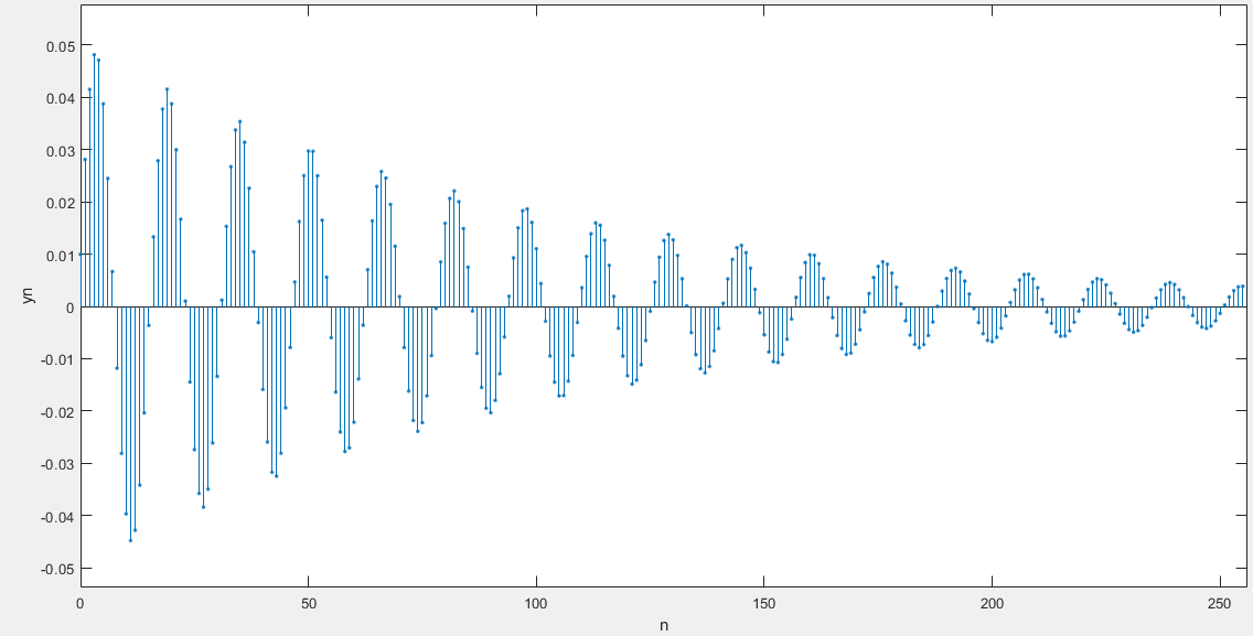
stable
Check the stability of the system
Add unit step sequence to the input and observe the waveform. If the waveform is stable at a constant value, the system is stable, otherwise it is unstable

Example 6

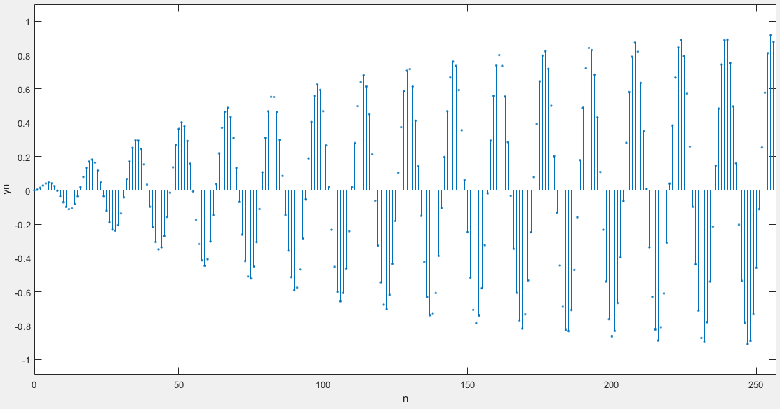
y(n)=1.8237y(n-1)-0.9801y(n-2)+1/100.49x(n)-1/100.49x(n-2)

The resonant frequency of the resonator is 0.4rad
The input signal is x(n)=sin(0.014* n)+sin(0.4*n), and the output is y(n)
Calculate the system output waveform

clc
close all;
clear all;
n=0:256;
xn=sin(0.014*n)+sin(0.4*n);
A=[1,-1.8237,0.9801];
B=[1/100.49,0,-1/100.49];
yn=filter(B,A,xn);
figure
stem(n,yn,'.');
xlabel('n');
ylabel('yn');
axis([0,length(n),1.2*min(yn),1.2*max(yn)]);

There are two methods to calculate the system response in time domain
1. Obtaining the system output through the difference equation requires the initial conditions and whether it is a zero input response
2. The system unit impulse response is known, and the system output is obtained by calculating the linear convolution between the input signal and the system unit impulse response

The resonator has the property of resonant to a certain frequency. The resonant frequency in the experiment is 0.4rad and the stable waveform is sin(0.4n)