catalogue
5, Experimental contents and results
1, Experiment name
matlab implementation of common sequences.
2, Experimental equipment
Computer with matlab software and textbook of digital signal processing course.
3, Experimental purpose
1. Master the basic operation and programming functions of matlab language;
2. Understand the graphics and implementation methods of common sequences, and master the programming method of generating common discrete-time signals by matlab;
3. Master the usage of basic functions exp, imag, real, two-dimensional graphics processing functions function, figure, stem, title, xlabel, ylabel, axis, grid on and general function graphics function subplot.
4, Experimental principle
1.matlab is powerful, easy to learn and has high programming efficiency. It has the functions of automatic control theory, digital signal processing, dynamic system simulation, image processing and so on;
2.matlab has a variety of function graphics processing and generators, which can process different functions, with fast analysis and calculation speed. It can use stem function to draw discrete graphics, which is very convenient to use;
3.matlab has powerful numerical calculation and symbolic calculation. It can easily draw two-dimensional, three-dimensional and four-dimensional graphics, and supports a variety of sound and image formats. The program can be run directly without compilation, which is very fast.
5, Experimental contents and results
The program generates unit impulse sequence, unit step sequence, rectangular sequence, real exponential sequence and complex exponential sequence, and draws its graph by using the basic graph function in matlab.
(1) Experiment 1: unit sampling sequence. In matlab, the unit sampling sequence can be realized by the following functions δ (n-n0) (as shown in Figure 1), it is realized by n==0.
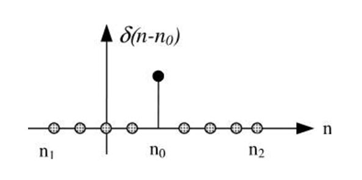
Figure 1 unit impulse sequence
- Experimental code
%Unit sampling sequence


function [x,n]=impseq(n0,n1,n2)       %produce x(n)=delta(n-n0);n1<=n0<=nn2

                                  %[x,n]=impseq(n0,n1,n2)

if((n0<n1)|(n0>n2)|(n1>n2))

    error('Parameters must meet n1<=n0<=n2')

end

n=[n1:n2];                        %x=[zeros(1,(n0-n1),1,zeros(1,(n2-n0))];

x=[(n-n0)==0];
2. Experimental results
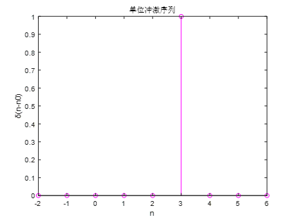
In the command window, do the following:
(1) Enter "n1=-2, n0=3, n2=6" and press enter;
(2) Enter "[x,n]=impseq(n0,n1,n2)" and press enter;
(3) Enter "stem(n,x)" and press enter. The results are as follows:
3. Problems encountered and Solutions
Problem: because the function function is used for the first time, I don't know much about the function function, and the initial values of input and output variables are not defined when running the result, so it can't run.
Solution: after running the program, enter n1=-2, n0=3, n2=6, enter [x,n]=impseq(n0,n1,n2), and finally enter stem(n,x) to run the result.
(2) Experiment 2: unit step sequence. In matlab, u(n-n0) can be realized with n > = 0 (as shown in Figure 2).
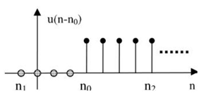
Figure 2 unit step sequence
1. Experimental code
%Unit Step Sequence


function [x,n]=stepseq(n0,n1,n2)        %produce x(n)=delta(n-n0);n1<=n0<=nn2

                                   %[x,n]=stepseq(n0,n1,n2)

if((n0<n1)|(n0>n2)|(n1>n2))

    error('Parameters must meet n1<=n0<=n2')

end

n=[n1:n2];                         %x=[zeros(1,(n0-n1),1,zeros(1,(n2-n0))];

x=[(n-n0)>=0];
2. Experimental results
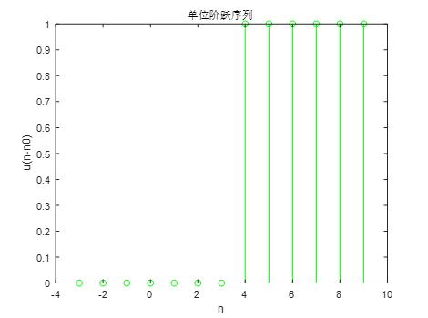
In the command window, do the following:
(1) Enter "n1=-4, n0=4, n2=10" and press enter;
(2) Enter "[x,n]=stepseq(n0,n1,n2)" and press enter;
(3) Enter "stem(n,x)" and press enter. The results are as follows:
(3) Experiment 3: rectangular sequence. In matlab, two unit step sequences can be subtracted to generate rectangular sequences (as shown in Figure 3).
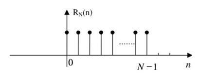
Figure 3 rectangular sequence
1. Experimental code
%Rectangular sequence


function [x1,x2,x3,n]=RN(n0,n1,n2)

if((n0<n1)|(n0>n2)|(n1>n2))

    error('Parameters must meet n1<=n0<=n2')

end

n=[n1:n2];

x1=[(n-n0)>=9];

x2=[(n-n0)>=-8];

x3=x2-x1;
2. Experimental results
In the command window, do the following:
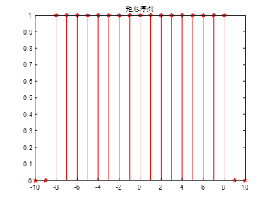
(1) Enter "n1=-10,n0=0,n2=10" and press enter;
(2) Enter "[x1,x2,x3,n]=RN(n0,n1,n2)" and press enter;
(3) Enter "stem(n,x3,'rp');title('rectangular sequence ');" enter. The results are as follows:
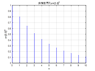
(4) Experiment 4: real exponential series. In matlab, the array operator '. ^' can be used to realize the real exponential sequence.
1. Experimental code
%Real exponential sequence


n=0:10;                       %definition n Scope of

x=(0.8).^n;

stem(n,x,'b.');               %Draw discrete image

title('Real exponential sequence x=(0.8)^n');  %Description of the image theme

xlabel('n');                  %Describe the horizontal axis

ylabel('x=(0.8)^n');          %Describe the longitudinal axis

grid on;                      %Open image grid
2. Experimental results
3. Problems encountered and Solutions
Problem: when writing code, the exponential function x=(0.8)^n was written less, and an error occurred when running the program.
Solution: change x=(0.8)^n to x=(0.8).^n, and then run again to get the result.
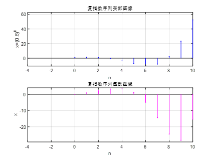
(5) Experiment 5: complex exponential sequence. Complex exponential sequence can be realized by programming in matlab 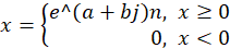 , where a=0.4, b=0.6.
1. Experimental code
%Complex exponential sequence


n=0:10;                       %definition n Scope of

x=exp((0.4+0.6j)*n);


%Generate real part image

subplot(2,1,1);               %Define the image window as 2 x1(2 Row 1 column),Coordinates are(1,1)(First row (first column)

stem(n,real(x),'b.');         %Draw a real discrete image and set the line to b((blue) dot Linetype

axis([-4,10,min(real(x))-1,1.2*max(real(x))]);      %Define the horizontal axis and vertical axis range of image 1

title('Real part image of complex exponential sequence');   %Description of the image theme

xlabel('n');                  %Describe the horizontal axis

ylabel('real(x)');            %Describe the longitudinal axis

grid on;                      %Open image grid


%Generate imaginary part image

subplot(2,1,2);               %Define the image window as 2 x2(2 Row 2 column),Coordinates are(2,1)(Second row (first column)

stem(n,imag(x),'m.');         %Draw an imaginary discrete image and set the line to m(Magenta) dot Linetype

axis([-4,10,min(imag(x))-1,1.2*max(imag(x))]);      %Define the horizontal axis and vertical axis range of image 2

title('Imaginary part image of complex exponential sequence');   %Description of the image theme

xlabel('n');                  %Describe the horizontal axis

ylabel('imag(x)');            %Describe the longitudinal axis

grid on;                      %Open image grid
2. Experimental results
6, Experimental harvest
Through this experiment, there are many unexpected gains, mainly including function knowledge and usage, image generation methods, and points needing attention during the experiment.
1. function knowledge: basic functions exp, imag, real, two-dimensional graphics processing functions
figure, stem, title, xlabel, ylabel, axis, grid on and general function graphic function subplot. These functions are very useful and important. They are basically useful in realizing general images.
2. Image generation method: there are three functions that can generate graphics, including function function and plot
Function and stem function.
3. Points needing attention during experiment
When using the function function, you should pay attention to:
1) Run the code program before assignment;
2) Assign a value to the input variable in the command window;
3) Then run for "[output] = file name (input)";
4) Finally, the graph is generated by stem function.
To generate graphics, you need to find out whether the graphics to be generated are continuous or discrete, and then select plot function (drawing continuous graphics) and stem function (drawing discrete graphics).
4. In short, as long as you are proactive, careful, patient, pay attention to integrating theory with practice, do more, learn more and ask more, you will make progress and learn more knowledge.