Drawing three-dimensional performance surfaces using Axes3D

Introduction: Drawing a 3D surface of a two-dimensional function can help us better understand the rules contained in the function. Axes3D is a drawing function in matplotlib. surface, countour,countourf, and so on can be used to display function 3D content very well.

Keywords: Axes3D, surface, contour, II

_01 Draw a surface

_Many times it is necessary to draw three-dimensional surface, such as drawing two-dimensional function values, optimizing the slice projection of the problem on two-dimensional, and so on. adopt Drawing meshgrid functions in classification interfaces and performance surfaces Or two-dimensional grid points can be calculated to draw three-dimensional surfaces and contours using surface, contour, and other functions.

1. Drawing Examples

1. Test Code

from headm import *                 #

from mpl_toolkits.mplot3d import Axes3D

x = arange(-4, 4, 0.1)
y = arange(-4, 4, 0.1)
x,y = meshgrid(x, y)
r = sqrt(x**2+y**2)
z = sin(r)

printt(z.shape\)

ax = Axes3D(plt.figure(figsize=(12,8)))
ax.plot_surface(x,y,z,rstride=1, cstride=2, cmap=plt.cm.hot)
ax.contour(x,y,z,
           zdir='z',
           offset=-2,
           cmap=plt.cm.hot)

ax.set_zlim(-2,2)
plt.show()

2. Test results

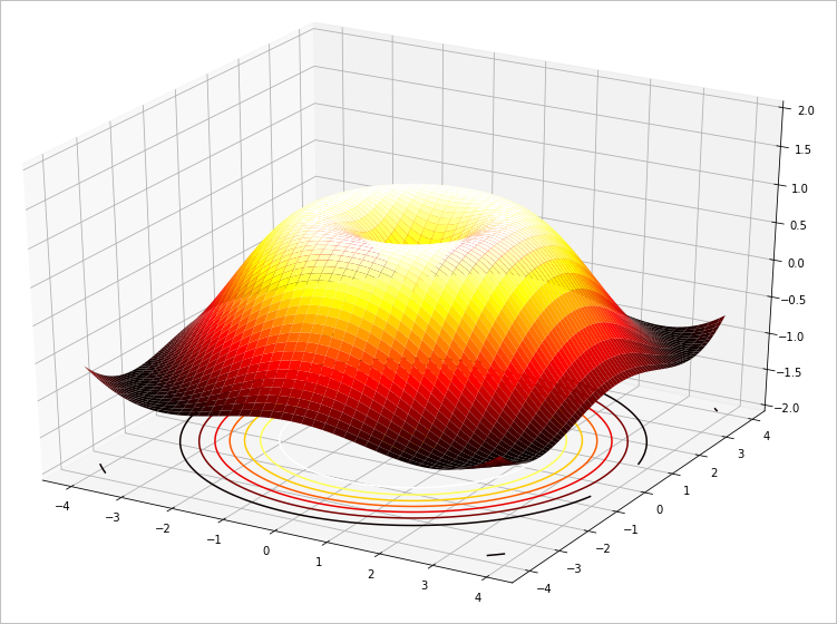
_Figure 1.1.1 plots a three-dimensional z-function

z.shape:(80, 80)

2. Color parameters

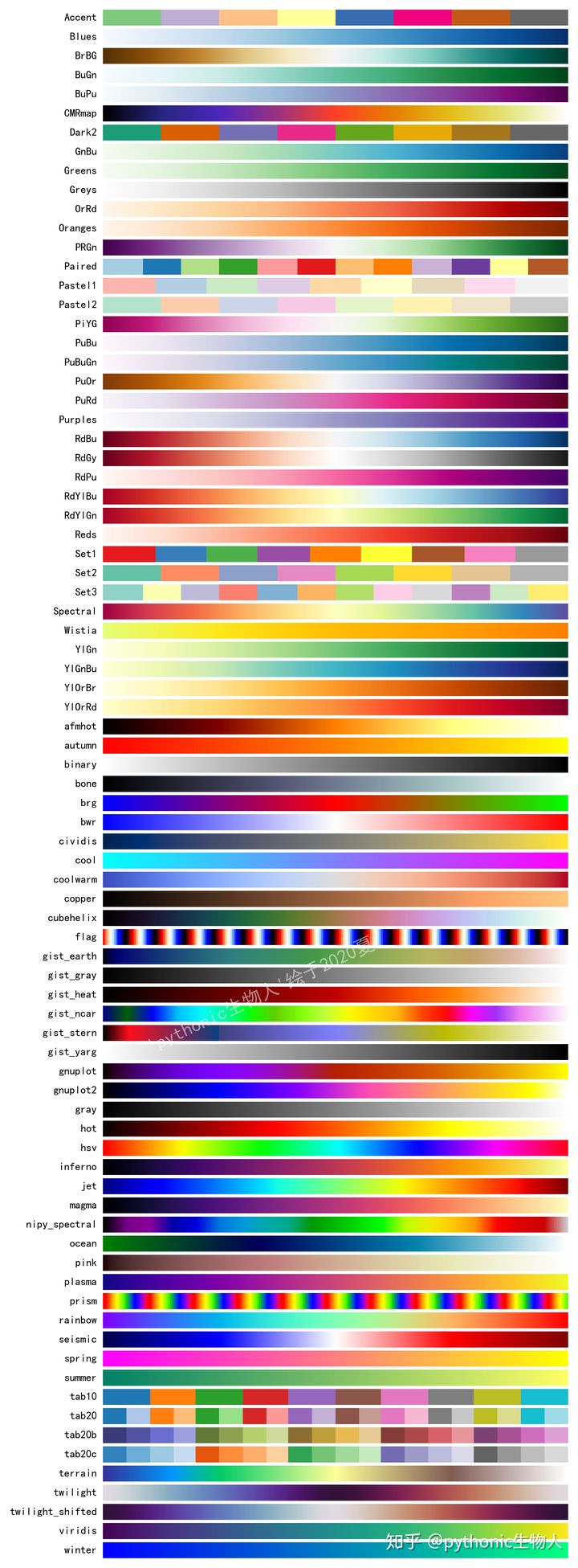
stay Python Visualization | matplotlib07 - Colormap with its own color bar (3) The various combinations of CMAPs are given.

1. Color Name

['Accent', 'Blues', 'BrBG', 'BuGn', 'BuPu', 'CMRmap', 'Dark2', 'GnBu', 'Greens', 'Greys', 'OrRd', 'Oranges', 'PRGn', 'Paired', 'Pastel1', 'Pastel2', 'PiYG', 'PuBu', 'PuBuGn', 'PuOr', 'PuRd', 'Purples', 'RdBu', 'RdGy', 'RdPu', 'RdYlBu', 'RdYlGn', 'Reds', 'Set1', 'Set2', 'Set3', 'Spectral', 'Wistia', 'YlGn', 'YlGnBu', 'YlOrBr', 'YlOrRd', 'afmhot', 'autumn', 'binary', 'bone', 'brg', 'bwr', 'cividis', 'cool', 'coolwarm', 'copper', 'cubehelix', 'flag', 'gist_earth', 'gist_gray', 'gist_heat', 'gist_ncar', 'gist_stern', 'gist_yarg', 'gnuplot', 'gnuplot2', 'gray', 'hot', 'hsv', 'inferno', 'jet', 'magma', 'nipy_spectral', 'ocean', 'pink', 'plasma', 'prism', 'rainbow', 'seismic', 'spring', 'summer', 'tab10', 'tab20', 'tab20b', 'tab20c', 'terrain', 'twilight', 'twilight_shifted', 'viridis', 'winter']

_Figure 1.2.1 colormap

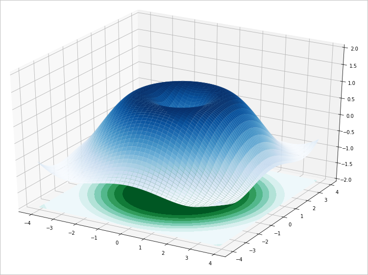
2. Change color

ax.plot_surface(x,y,z,rstride=1, cstride=2, cmap=plt.cm.Blues)
ax.contourf(x,y,z,
           zdir='z',
           offset=-2,
           cmap=plt.cm.BuGn)

_Fig.1.2.2 Altitude after color change

_02 More examples

1. Combination of resistors

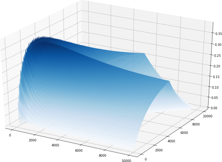
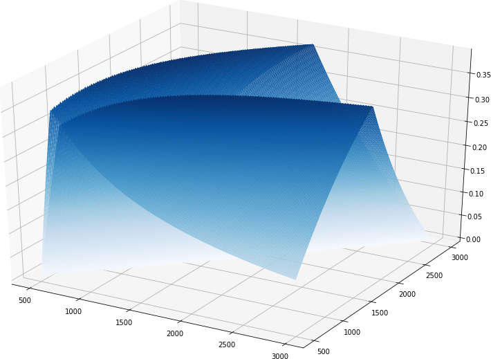
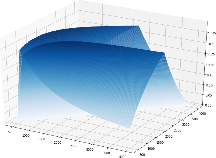
_In Read multiple buttons through one port When searching for multiple resistor parallel switches, the corresponding maximum voltage interval. You can see that the peaks are very complex. The following searches for a combination of two resistors to draw a performance surface.

1. Search Code

R0                     = 1e3
U0                     = 3.3
def minVoltage(r1,r2):
    rdim = [10e10, r1, r2,
            1/(1/r1 + 1/r2)]
    vdim = sorted([r/(r+R0)*U0 for r in rdim])
    vdiff = [b-a for a,b in zip(vdim[:-1], vdim[1:])]
    vdiff.append(vdim[0])

    return min(vdiff)

STEP_NUM        = 50
x = arange(100, 10000, STEP_NUM)
y = arange(100, 10000, STEP_NUM)
x,y = meshgrid(x, y)

z = array([minVoltage(x,y) for x,y in zip(x.flatten(), y.flatten())]).reshape(x.shape)

2. Search results

(1) Search scope: 100:10000:50

_Figure 2.1.1 Searches for performance curves for R1,R2

(2) Search range: 500:3000:10

_Figure 2.1.2 Searches for R1,R2 performance curves

(3) Search range: 500:4000:10

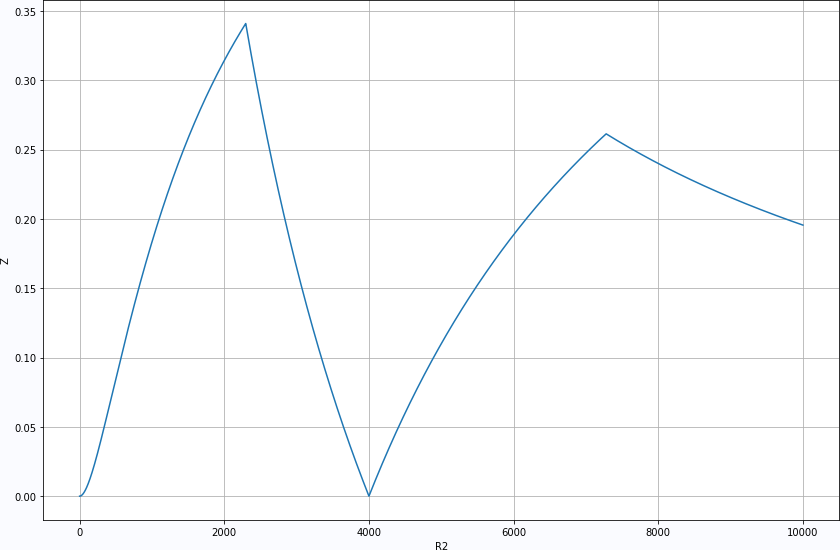
_Figure 2.1.3 Searches for R1,R2 performance curves

3. Slice to one dimension

R1 = 4e3
R2 = linspace(0, 10000, 10000)
z = [minVoltage(R1, r2) for r2 in R2]
plt.clf()
plt.figure(figsize=(12,8))
plt.plot(R2, z)
plt.xlabel("R2")
plt.ylabel("Z")
plt.grid(True)
plt.tight_layout()

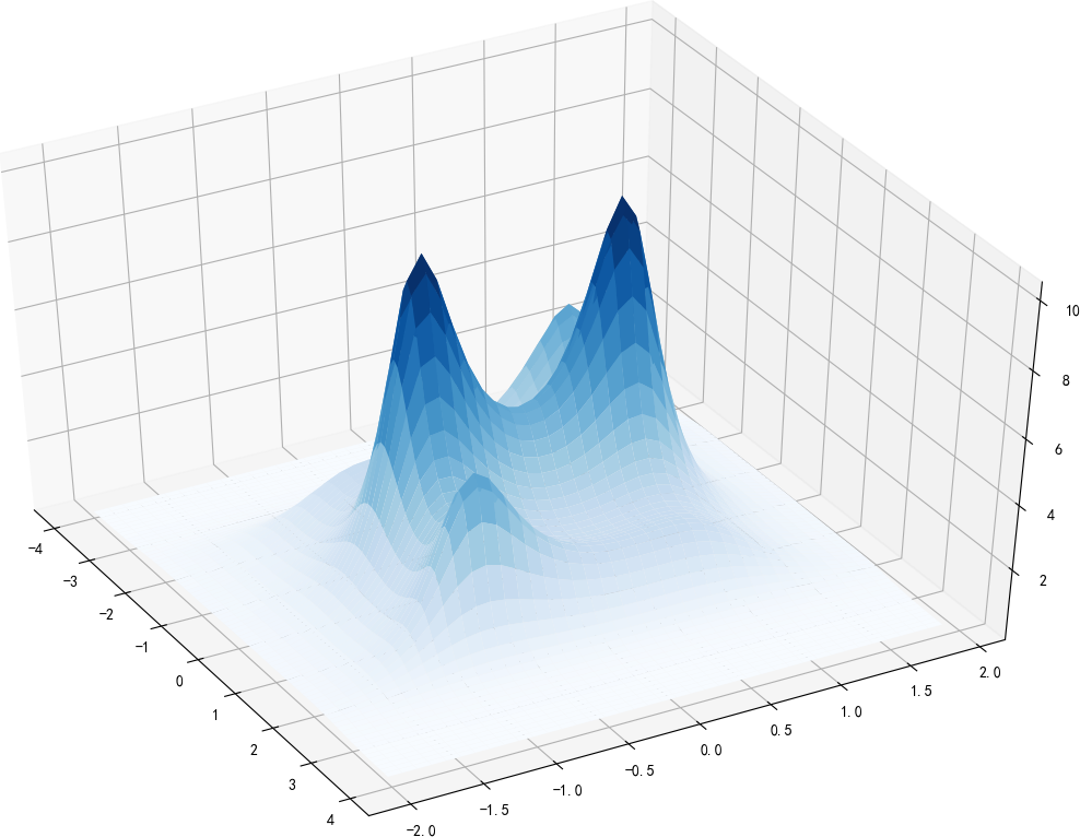
_Maximum voltage corresponding to Figure 2.1.4 R2

2. 2-D Nonlinear Functions

f = 10 4 x 1 2 − 2.1 x 1 4 + 1 3 x 1 6 + x 1 x 2 − 4 x 2 2 + 4 x 2 2 + 2 f = {{10} \over {4x_1^2 - 2.1x_1^4 + {1 \over 3}x_1^6 + x_1 x_2 - 4x_2^2 + 4x_2^2 + 2}} f=4x12−2.1x14+31x16+x1x2−4x22+4x22+210

x = arange(-4, 4, 0.1)
y = arange(-2, 2, 0.1)
x,y = meshgrid(x,y)
z = 10/(4*x**2 - 2.1*x**4 + x**6/3 + x*y - 4*y**2+4*y**4 + 2)

print(z.shape)

ax = Axes3D(plt.figure(figsize=(12,8)))
ax.plot_surface(x,y,z,
                rstride=1,
                cstride=1,
                cmap=plt.cm.Blues)

plt.show()

_Figure 2.2.1 Drawn 3D Image

_total_knot_

_Drawing a 3D surface of a two-dimensional function can help us better understand the rules contained in the function. Axes3D is a drawing function in matplotlib. surface, countour,countourf, and so on can be used to display function 3D content very well.

Links to related literature:

Programming VIP