Introduction to Dropout

1.1 Reasons for Dropout

_In the machine learning model, if there are too many parameters of the model and too few training samples, the trained model can easily be fitted. When training the neural network, we often encounter the problem of fitting, which is manifested in the following aspects: the loss function of the model on the training data is small, and the prediction accuracy is high; However, on the test data, the loss function is larger and the prediction accuracy is lower.

Over-fitting is a common problem in many machine learning. If the model fits too well, the resulting model is hardly usable. In order to solve the problem of fitting, a method of model integration is usually used, that is, training multiple models to combine. At this time, the training model time-consuming becomes a big problem, not only training multiple models time-consuming, but also testing multiple models time-consuming.

To sum up, there are always two drawbacks when training deep neural networks:

Easy over-fitting
Time-consuming

Dropout can alleviate the occurrence of over-fitting effectively and achieve regularization to some extent.

1.2 What is Dropout

_In 2012, Hinton proposed Dropout in his paper Improving neural networks by preventing co-adaptation of feature detectors. When a complex feed-forward neural network is trained in small datasets, it is easy to overfit. To prevent overfitting, the performance of the neural network can be improved by preventing the interaction of the feature detectors.

_In 2012, Alex and Hinton used the Dropout algorithm in their paper ImageNet Classification with Deep Convolutional Neural Networks to prevent over-fitting. Moreover, the AlexNet network model mentioned in this paper has triggered a boom in the application of neural networks and won the 2012 Image Recognition Contest, making CNN the core algorithm model in image classification.

_Subsequently, there were several articles about Dropout, Dropout:A Simple Way to Prevent Neural Networks from Overfitting, Improving Neural Networks with Dropout, and Dropout data augmentation.

_From the above paper, we can feel the importance of Dropout in deep learning. So, what exactly is Dropout?

_Dropout can be used as a trick for training depth neural networks. In each training batch, overfitting can be significantly reduced by ignoring half of the feature detectors (with half of the hidden layer nodes having a value of 0). This approach reduces the interaction between feature detectors (hidden layer nodes), which means that some detectors rely on other detectors to function.

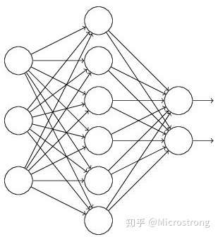
One simple point Dropout says is that when we propagate forward, we stop a neuron's activation value at a certain probability p, which makes the model more generalized because it does not rely too much on certain local characteristics, as shown in Figure 1.

2. Dropout workflow and use

2.1 Dropout specific workflow

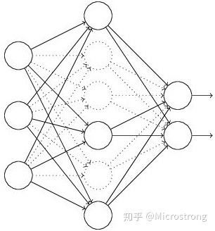
Suppose we want to train such a neural network, as shown in Figure 2.

_Input is x output is y, the normal flow is: we first propagate x forward through the network, and then reverse propagate the error to determine how to update the parameters for the network to learn. After using Dropout, the process becomes as follows:

_First, half of the hidden neurons in the network are randomly (temporarily) deleted, while the input and output neurons remain unchanged (the dashed line in Figure 3 is a partially temporarily deleted neuron).

_Then the input x is propagated forward through the modified network, and the loss result is propagated back through the modified network. After a small batch of training samples completes this process, the corresponding parameters (w, b) are updated according to the random gradient descent method on the undeleted neurons.

_Then continue the process:

• Restore deleted neurons (at this point deleted neurons remain as they were, and those that were not deleted have been updated)
• A half-sized subset of the hidden layer neurons is randomly selected for temporary deletion (backing up the parameters of the deleted neurons).
• For a small number of training samples, the loss is propagated to and then propagated back, and the parameters (w, b) are updated according to the random gradient descent method (the part of the parameters that are not deleted is updated, and the deleted neuron parameters remain the results before they are deleted).

Repeat this process over and over again.

2.2 Use of Dropout in Neural Networks

_Dropout's specific workflow has been described in detail above, but how can certain neurons stop working at a certain probability (that is, they are deleted)? How does the code level work?

_Below, we will specifically explain some of the Dropout code level formula derivation and code implementation ideas.

(1) In the training model stage

Inevitably, a probability process is added to each unit of the training network.

The corresponding formula changes as follows:

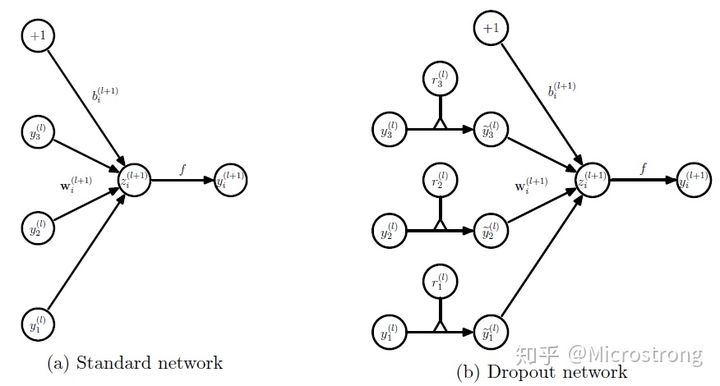
• Network calculation formula without Dropout:
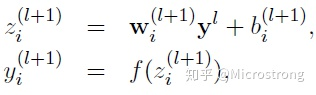
• Using Dropout's network calculation formula:
  

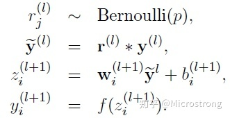
_The Bernoulli function in the above formula is used to generate a probability r vector, that is, a random vector of 0 and 1.

_Code level allows a neuron to stop working with probability p, essentially changing its activation function value to zero with probability P. For example, if the number of neurons in one layer of our network is 1000, and the output values of the activation function are y1, y2, y3,..., y1000, and our dropout ratio is 0.4, then after dropout, about 400 out of 1000 neurons will be set to zero.

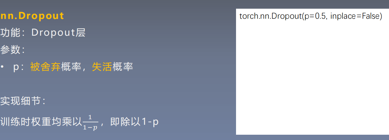
_Note: After blocking some neurons above and making them active at 0, we also need to scale the vector y1...y1000, which is multiplied by 1/(1-p). If you did not rescale y1...y1000 after setting 0 during training, you will need to scale the weight during testing as follows.
(2) In the testing model phase

When predicting a model, the weight parameter for each neuron unit is multiplied by the probability p.

Dropout formula for test phase:
W t e s t l W^{l} _{test} Wtestl​ = p W l pW^l pWl

3. Why does Dropout solve the fit?

Average effect:
_Back to the standard model without dropout, we use the same training data to train five different neural networks and generally get five different results. At this time, we can use "five result mean" or "majority winning voting strategy" to determine the final result. For example, if the result of three networks is number 9, it is likely that the real result is number 9, and the other two networks give incorrect results. This "aggregated averaging" strategy often prevents over-fitting problems. Since different networks may produce different overfitting, averaging may cancel out some "opposite" fitting. Dropout removes different hidden neurons like training different networks. Randomly removing half of the hidden neurons results in different network structures. The entire dropout process is equivalent to averaging many different networks. Different networks produce different overfitting, some of which are "reverse" to offset each other can reduce overfitting as a whole.

Reducing complex co-adaptive relationships between neurons:
_Because the dropout program results in two neurons not necessarily appearing in one dropout network at a time. In this way, the updating of weights is no longer dependent on the joint action of implicit nodes with fixed relationships, which prevents some features from being effective only under other specific features. The network is forced to learn more robust features, which also exist in a random subset of other neurons. In other words, if our neural network is making some predictions, it should not be overly allergic to certain segments of clues, and even if a particular clue is lost, it should be able to learn some common traits from many other clues. From this point of view, dropout is a bit like the L1, L2 rule, and reducing weights improves the robustness of the network to lose specific neuron connections.

Dropout is similar to the role of gender in biological evolution:
_Species tend to adapt to this environment in order to survive. Environmental mutations can make it difficult for species to respond in a timely manner. The emergence of sex can result in varieties adapted to new environments, effectively preventing overfitting, i.e. avoiding extinction when the environment changes.

4. Source Code Analysis of Dropout in Pytorch

import torch
import torch.nn as nn
import matplotlib.pyplot as plt
import sys, os
hello_pytorch_DIR = os.path.abspath(os.path.dirname(__file__)+os.path.sep+".."+os.path.sep+"..")
sys.path.append(hello_pytorch_DIR)

from PYTORCH.Deep_eye.Pytorch_Camp_master.hello_pytorch.tools.common_tools import set_seed
from torch.utils.tensorboard import SummaryWriter

set_seed(1)  # Set up random seeds
n_hidden = 200
max_iter = 2000
disp_interval = 400
lr_init = 0.01


# ===================================== step 1/5 data===========================
def gen_data(num_data=10, x_range=(-1, 1)):

    w = 1.5
    train_x = torch.linspace(*x_range, num_data).unsqueeze_(1)
    train_y = w*train_x + torch.normal(0, 0.5, size=train_x.size())
    test_x = torch.linspace(*x_range, num_data).unsqueeze_(1)
    test_y = w*test_x + torch.normal(0, 0.3, size=test_x.size())

    return train_x, train_y, test_x, test_y


train_x, train_y, test_x, test_y = gen_data(x_range=(-1, 1))


# ===================================== step 2/5 model===========================
# Dropout is not normally added before the output layer
class MLP(nn.Module):
    def __init__(self, neural_num, d_prob=0.5):
        super(MLP, self).__init__()
        self.linears = nn.Sequential(

            nn.Linear(1, neural_num),
            nn.ReLU(inplace=True),

            nn.Dropout(d_prob),
            nn.Linear(neural_num, neural_num),
            nn.ReLU(inplace=True),

            nn.Dropout(d_prob),
            nn.Linear(neural_num, neural_num),
            nn.ReLU(inplace=True),

            nn.Dropout(d_prob),
            nn.Linear(neural_num, 1),
        )

    def forward(self, x):
        return self.linears(x)


net_prob_0 = MLP(neural_num=n_hidden, d_prob=0.)  # d_prob=0. Do not Dropout
net_prob_05 = MLP(neural_num=n_hidden, d_prob=0.5) # Dropout probability 0.5

# ====================================== step 3/5 optimizer==========================
optim_normal = torch.optim.SGD(net_prob_0.parameters(), lr=lr_init, momentum=0.9)
optim_reglar = torch.optim.SGD(net_prob_05.parameters(), lr=lr_init, momentum=0.9)

# ======================================= step 4/5 loss function=========================
loss_func = torch.nn.MSELoss()

# ======================================= step 5/5 iteration training=========================

writer = SummaryWriter(comment='_test_tensorboard', filename_suffix="12345678")
for epoch in range(max_iter):

    pred_normal, pred_wdecay = net_prob_0(train_x), net_prob_05(train_x)
    loss_normal, loss_wdecay = loss_func(pred_normal, train_y), loss_func(pred_wdecay, train_y)

    optim_normal.zero_grad()
    optim_reglar.zero_grad()

    loss_normal.backward()
    loss_wdecay.backward()

    optim_normal.step()
    optim_reglar.step()

    if (epoch+1) % disp_interval == 0:

        net_prob_0.eval() # net uses test status
        net_prob_05.eval()

        # visualization
        for name, layer in net_prob_0.named_parameters():
            writer.add_histogram(name + '_grad_normal', layer.grad, epoch)
            writer.add_histogram(name + '_data_normal', layer, epoch)

        for name, layer in net_prob_05.named_parameters():
            writer.add_histogram(name + '_grad_regularization', layer.grad, epoch)
            writer.add_histogram(name + '_data_regularization', layer, epoch)

        test_pred_prob_0, test_pred_prob_05 = net_prob_0(test_x), net_prob_05(test_x)

        # Mapping
        plt.clf()
        plt.scatter(train_x.data.numpy(), train_y.data.numpy(), c='blue', s=50, alpha=0.3, label='train')
        plt.scatter(test_x.data.numpy(), test_y.data.numpy(), c='red', s=50, alpha=0.3, label='test')
        plt.plot(test_x.data.numpy(), test_pred_prob_0.data.numpy(), 'r-', lw=3, label='d_prob_0')
        plt.plot(test_x.data.numpy(), test_pred_prob_05.data.numpy(), 'b--', lw=3, label='d_prob_05')
        plt.text(-0.25, -1.5, 'd_prob_0 loss={:.8f}'.format(loss_normal.item()), fontdict={'size': 15, 'color': 'red'})
        plt.text(-0.25, -2, 'd_prob_05 loss={:.6f}'.format(loss_wdecay.item()), fontdict={'size': 15, 'color': 'red'})

        plt.ylim((-2.5, 2.5))
        plt.legend(loc='upper left')
        plt.title("Epoch: {}".format(epoch+1))
        plt.show()
        plt.close()

        net_prob_0.train()
        net_prob_05.train()

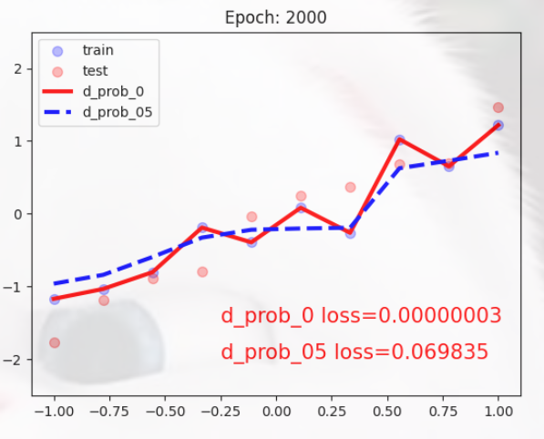
The Loss of the red line is very low and is completely over-fitted.
By adding Dropout to the blue curve, the overfitting is significantly reduced and the curve is smoother.

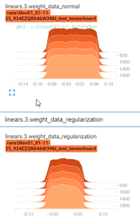
Dropout controls the scale of weight: (function of shrinking weight)
dropout produces the effect of shrinking the square norm of the weights, similar to L2 regularization, which results in compressing the weights and completing some outer regularization that prevents overfitting.

import torch
import torch.nn as nn
import matplotlib.pyplot as plt
import sys, os
hello_pytorch_DIR = os.path.abspath(os.path.dirname(__file__)+os.path.sep+".."+os.path.sep+"..")
sys.path.append(hello_pytorch_DIR)

from PYTORCH.Deep_eye.Pytorch_Camp_master.hello_pytorch.tools.common_tools import set_seed
from torch.utils.tensorboard import SummaryWriter

# set_seed(1)  # Set up random seeds


class Net(nn.Module):
    def __init__(self, neural_num, d_prob=0.5):
        super(Net, self).__init__()

        self.linears = nn.Sequential(

            nn.Dropout(d_prob),
            nn.Linear(neural_num, 1, bias=False),
            nn.ReLU(inplace=True)
        )

    def forward(self, x):
        return self.linears(x)

input_num = 10000
x = torch.ones((input_num, ), dtype=torch.float32)

net = Net(input_num, d_prob=0.5)
net.linears[1].weight.detach().fill_(1.)

net.train()
y = net(x)
print("output in training mode", y)

net.eval()
y = net(x)
print("output in eval mode", y)

OUT:

output in training mode tensor([9982.], grad_fn=<ReluBackward0>)
output in eval mode tensor([10000.], grad_fn=<ReluBackward0>)

Note: The implementation of Dropout in Keras is to block out some neurons so that after their activation value is 0, the activation vector x1...x1000 is amplified, that is, multiplied by 1/(1-p).

Reflection:

_We have described two ways to zoom Dropout, so why does Dropout need to zoom?

_Because we randomly discard some neurons during training, but we can't discard them randomly when predicting. If some neurons are discarded, the result will be unstable, that is, given a test data, sometimes output a and sometimes output b, the result will be unstable, which is unacceptable to the actual system, users may think the model prediction is inaccurate. A compensatory scheme would then be to multiply the weight of each neuron by a p, so that the test and training data would be roughly the same overall. For example, if the output of a neuron is x, it has the probability of P participating in the training at the time of training, (1-p) discarded, then the expected output of a neuron is p x+ (1-p) 0=p X. So multiplying the weight of this neuron by P during the test would give you the same expectation.

Summary:

_Dropout is currently heavily used in fully connected networks and is generally considered to be set to 0.5 or 0.3. In the convolution network hidden layer, Dropout strategy is less used in the convolution network hidden layer due to the sparseness of the convolution itself and the large use of sparse ReLu function. Overall, Dropout is a super-parameter, which needs to be tried according to the specific network and specific application areas.