Produced by CDA Data Analyst Author: CDA teaching and Research Group Editor: Mika
Case introduction
Background: Taking the user behavior data of a large e-commerce platform as the data set, the user behavior characteristics under massive data are analyzed by using big data processing technology, and the user behavior is predicted by establishing logistic regression model and random forest;
Case ideas:
- Using big data processing technology to read massive data
- Massive data preprocessing
- Extract part of data debugging model
- Building models with massive data
#All row output
from IPython.core.interactiveshell import InteractiveShell InteractiveShell.ast_node_interactivity = "all"
Data dictionary:
U_Id:the serialized ID that represents a user
T_Id:the serialized ID that represents an item
C_Id:the serialized ID that represents the category which the corresponding item belongs to Ts:the timestamp of the behavior
Be_type:enum-type from ('pv', 'buy', 'cart', 'fav')
pv: Page view of an item's detail page, equivalent to an item click
buy: Purchase an item
cart: Add an item to shopping cart fav: Favor an item
Read data
The key here is to use dask library to process massive data. Most of its operations run about ten times faster than conventional pandas and other libraries.
Pandas is very popular and powerful in analyzing structured data, but its biggest limitation is that scalability is not considered in the design. Pandas is especially suitable for dealing with small structured data, and is highly optimized to perform fast and efficient operations on the data stored in memory. However, with the substantial increase in the amount of data, a single machine will certainly not be able to read. Cluster processing is the best choice. This is where the Dask DataFrame API works: by providing a wrapper for pandas, you can intelligently separate huge dataframes into smaller fragments, disperse them into multiple workers (frames), and store them on disk instead of RAM.
Dask DataFrame will be divided into multiple departments. Each part is called a partition. Each partition is a relatively small DataFrame, which can be assigned to any worker and maintain its complete data when replication is needed. The specific operation is to operate each partition in parallel or separately (multiple machines can also be parallel), and then merge the results. In fact, it can be inferred intuitively that dask must do so.
# Installation Library (Tsinghua image)
# pip install dask -i https://pypi.tuna.tsinghua.edu.cn/simple
import os
import gc # Garbage collection interface
from tqdm import tqdm # Progress bar library
import dask # Parallel computing interface
from dask.diagnostics import ProgressBar
import numpy as np
import pandas as pd
import matplotlib.pyplot as plt
import time
import dask.dataframe as dd # dask Data table processing library in import sys # External parameter acquisition interface
In the face of massive data, you can add a line of GC after running a module Collect() to recycle memory fragments. Dask Dataframes and Pandas Dataframes have the same API
gc.collect()
42
# Load data
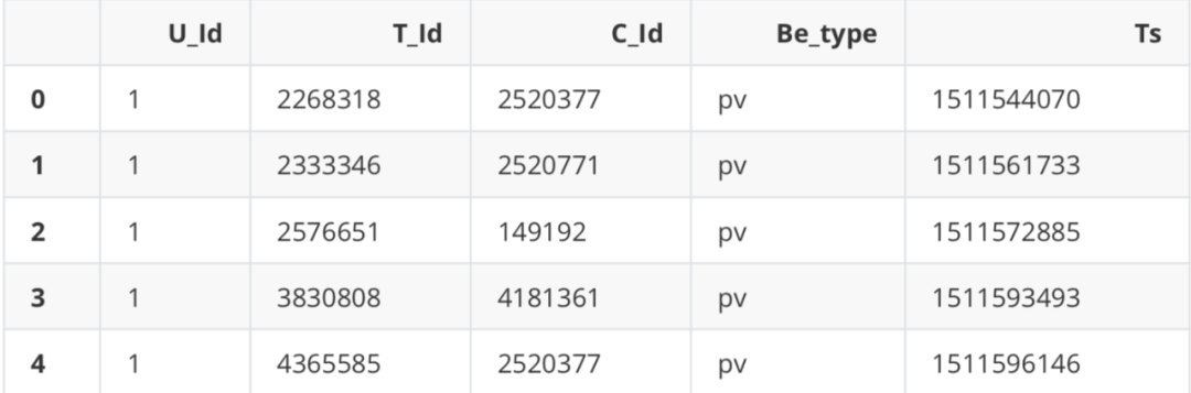
data = dd.read_csv('UserBehavior_all.csv')# If necessary, you can set the blocksize = parameter to manually specify the partition method. The default is 64MB (it needs to be set as a multiple of the bus, otherwise it will slow down)
data.head()
.dataframe tbody tr th {
    vertical-align: top;
}
.dataframe thead th {
    text-align: right;
}
data
Dask DataFrame Structure :
.dataframe tbody tr th {
    vertical-align: top;
}
.dataframe thead th {
    text-align: right;
}
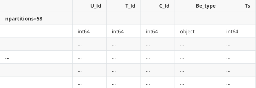
Dask Name: read-csv, 58 tasks
Unlike pandas, we only get the structure of the data frame here, not the actual data frame. Dask has loaded the data frame into several blocks, which exist on disk but not in RAM. If you have to output data frames, you first need to put all data frames into RAM, sew them together, and then display the final data frame. use. Compute () forces it to do so, otherwise it won't compute() . In fact, dask uses a delayed data loading mechanism, which is similar to the iterator component of python. It will actually load data only when data needs to be used.
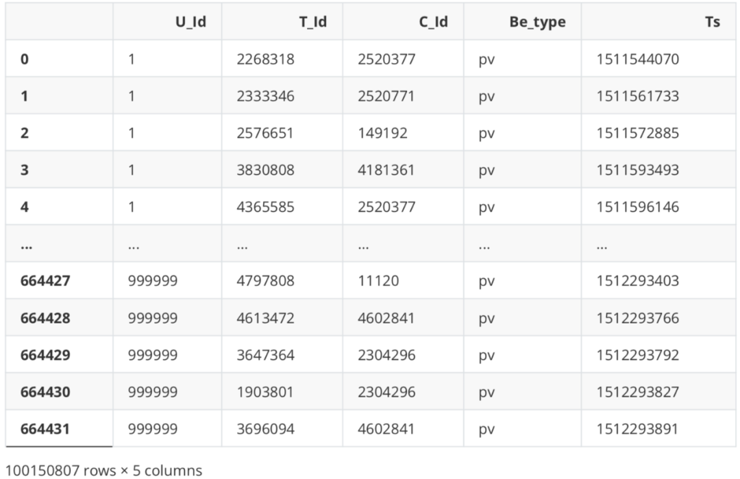
# Really load data compute()
.dataframe tbody tr th {
    vertical-align: top;
}
.dataframe thead th {
    text-align: right;
}
# Visual work process, 58 partition tasks, data visualize()
Data preprocessing
data compression
# View the current data type data dtypes
U_Id        int64
T_Id        int64
C_Id        int64
Be_type    object
Ts          int64
dtype: object
# Compressed into 32-bit uint, unsigned integer, because the transaction data has no negative number dtypes ={
    'U_Id': 'uint32',
    'T_Id': 'uint32',
    'C_Id': 'uint32',
    'Be_type': 'object',
    'Ts': 'int64'
}
data = data.astype(dtypes)
data.dtypes
U_Id       uint32
T_Id       uint32
C_Id       uint32
Be_type    object
Ts          int64
dtype: object
Missing value
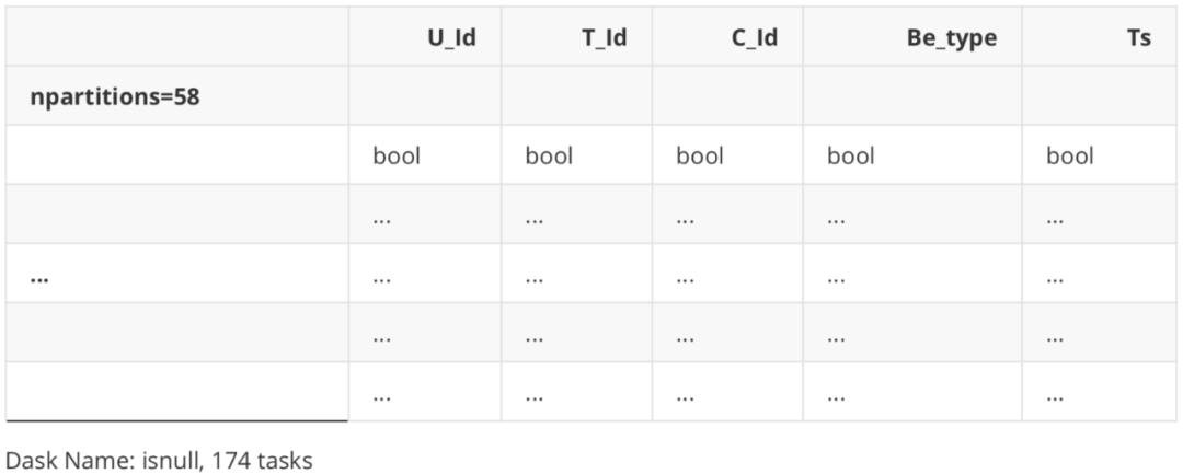
# The data read by dask interface cannot be used directly Common pandas functions such as isnull () screen for missing data isnull()
Dask DataFrame Structure :
.dataframe tbody tr th {
    vertical-align: top;
}
.dataframe thead th {
    text-align: right;
}
columns1 = [ 'U_Id', 'T_Id', 'C_Id', 'Be_type', 'Ts']
tmpDf1 = pd.DataFrame(columns=columns1)
tmpDf1
.dataframe tbody tr th {
    vertical-align: top;
}
.dataframe thead th {
    text-align: right;
}

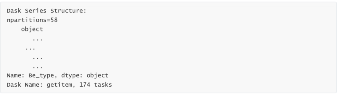
s = data["U_Id"].isna()
s.loc[s == True]
Dask Series Structure:
npartitions=58
bool ...
... ...
     ...
Name: U_Id, dtype: bool
Dask Name: loc-series, 348 tasks
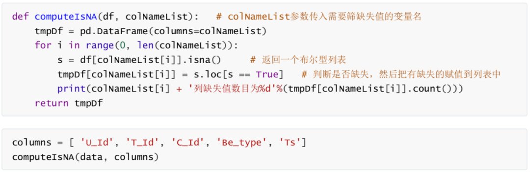
U_Id The number of column missing values is 0
T_Id The number of column missing values is 0
C_Id The number of column missing values is 0
Be_type The number of column missing values is 0
Ts The number of column missing values is 0
.dataframe tbody tr th {
    vertical-align: top;
}
.dataframe thead th {
    text-align: right;
}

No missing values
Data exploration and visualization
Here we use the pyecarts library. Pyecarts is a data visualization tool that combines python with Baidu's open source ecarts. New version 1 X and older versions of 0.5 The code rules of version x are very different. See the official documents for the new version https://gallery.py echarts.org/#/README
# pip install pyecharts -i https://pypi.tuna.tsinghua.edu.cn/simple
Looking in indexes: https://pypi.tuna.tsinghua.edu.cn/simple
Requirement already satisfied: pyecharts in d:\anaconda\lib\site-packages (0.1.9.4)
Requirement already satisfied: jinja2 in d:\anaconda\lib\site-packages (from pyecharts)
(3.0.2)
Requirement already satisfied: future in d:\anaconda\lib\site-packages (from pyecharts)
(0.18.2)
Requirement already satisfied: pillow in d:\anaconda\lib\site-packages (from pyecharts)
(8.3.2)
Requirement already satisfied: MarkupSafe>=2.0 in d:\anaconda\lib\site-packages (from
jinja2->pyecharts) (2.0.1)
Note: you may need to restart the kernel to use updated packages.
U_Id The number of column missing values is 0 T_Id The number of column missing values is 0 C_Id The number of column missing values is 0 Be_type The number of column missing values is 0 Ts The number of column missing values is 0
WARNING: Ignoring invalid distribution -umpy (d:\anaconda\lib\site-packages)
WARNING: Ignoring invalid distribution -ip (d:\anaconda\lib\site-packages)
WARNING: Ignoring invalid distribution -umpy (d:\anaconda\lib\site-packages)
WARNING: Ignoring invalid distribution -ip (d:\anaconda\lib\site-packages)
WARNING: Ignoring invalid distribution -umpy (d:\anaconda\lib\site-packages)
WARNING: Ignoring invalid distribution -ip (d:\anaconda\lib\site-packages)
WARNING: Ignoring invalid distribution -umpy (d:\anaconda\lib\site-packages)
WARNING: Ignoring invalid distribution -ip (d:\anaconda\lib\site-packages)
WARNING: Ignoring invalid distribution -umpy (d:\anaconda\lib\site-packages)
WARNING: Ignoring invalid distribution -ip (d:\anaconda\lib\site-packages)
Pie chart
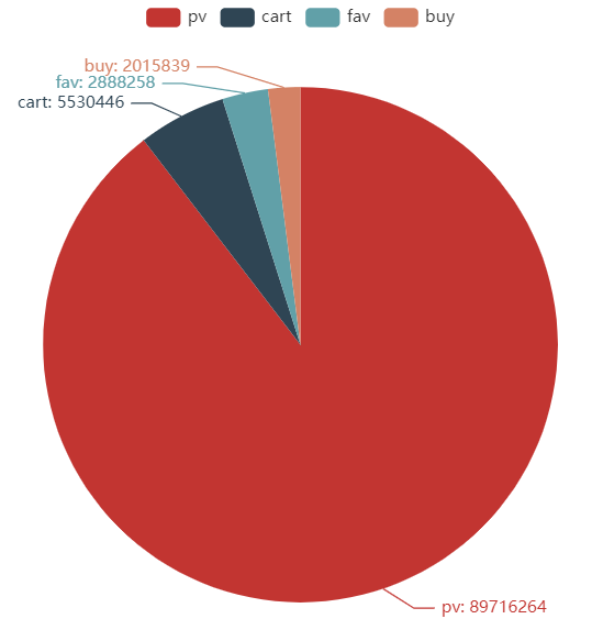
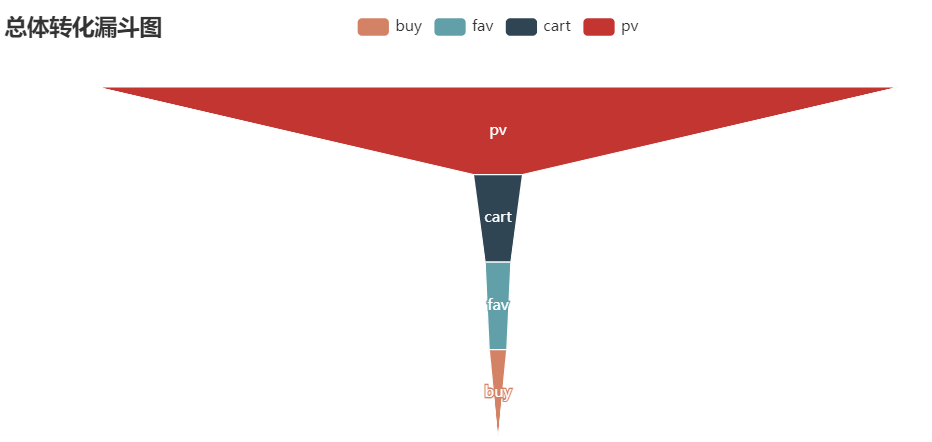
# For example, we want to draw a beautiful pie chart to see the proportion of various user behaviors data["Be_type"]
# When using dask, all supported original pandas functions need to be added compute() for final execution
Be_counts = data["Be_type"].value_counts().compute()
Be_counts
pv      89716264
cart     5530446
fav      2888258
buy      2015839
Name: Be_type, dtype: int64
Be_index = Be_counts.index.tolist() # Extract label
Be_index
['pv', 'cart', 'fav', 'buy']
Be_values = Be_counts.values.tolist() # Extract value
Be_values
[89716264, 5530446, 2888258, 2015839]
from pyecharts import options as opts
from pyecharts.charts import Pie
#The data in the pie package must be passed into a list of tuples
c = Pie()
c.add("", [list(z) for z in zip(Be_index, Be_values)]) # zip The iteratable object() function packages iteratable objects into tuples and returns a list of tuples c.set_global_opts(title_opts=opts.TitleOpts(title="User behavior")) # Global parameter (Figure naming) c.set_series_opts(label_opts=opts.LabelOpts(formatter="{b}: {c}"))
c.render_notebook() # Output to current notebook environment
# c.render("pie_base.html") # If necessary, you can output the diagram to this machine
<pyecharts.charts.basic_charts.pie.Pie at 0x1b2da75ae48>
<div id="490361952ca944fcab93351482e4b254" style="width:900px; height:500px;"></div>
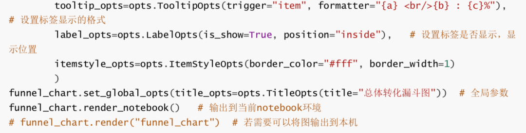
Funnel diagram
from pyecharts.charts import Funnel # The old version of pyecarts is not required Import pyechards options as opts
from IPython.display import Image as IMG
from pyecharts import options as opts
from pyecharts.charts import Pie
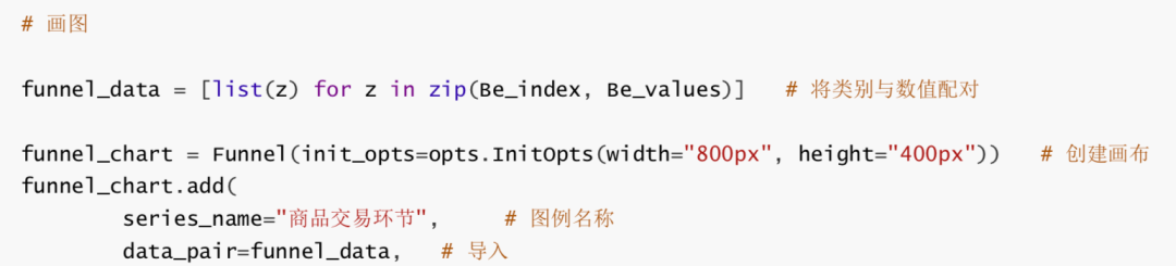
<pyecharts.charts.basic_charts.funnel.Funnel at 0x1b2939d50c8>
<div id="071b3b906c27405aaf6bc7a686e36aaa" style="width:800px; height:400px;"></div>
Data analysis
Timestamp conversion
dask's support for timestamps is very unfriendly
type(data)
dask.dataframe.core.DataFrame
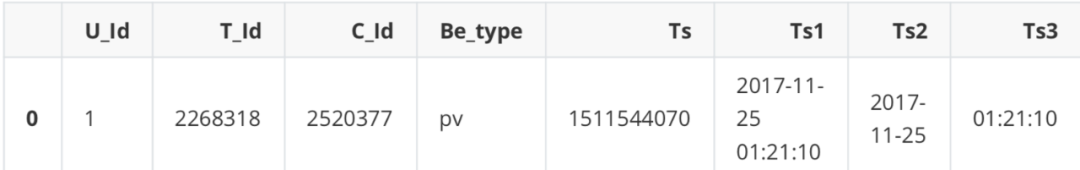
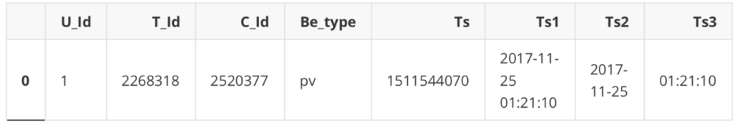
data['Ts1']=data['Ts'].apply(lambda x: time.strftime("%Y-%m-%d %H:%M:%S",
time.localtime(x)))
data['Ts2']=data['Ts'].apply(lambda x: time.strftime("%Y-%m-%d", time.localtime(x)))
data['Ts3']=data['Ts'].apply(lambda x: time.strftime("%H:%M:%S", time.localtime(x)))
D:\anaconda\lib\site-packages\dask\dataframe\core.py:3701: UserWarning:
You did not provide metadata, so Dask is running your function on a small dataset to
guess output types. It is possible that Dask will guess incorrectly.
To provide an explicit output types or to silence this message, please provide the
`meta=` keyword, as described in the map or apply function that you are using.
  Before: .apply(func)
  After:  .apply(func, meta=('Ts', 'object'))
  warnings.warn(meta_warning(meta))
data.head(1)
.dataframe tbody tr th {
    vertical-align: top;
}
.dataframe thead th {
    text-align: right;
}
data.dtypes
U_Id       uint32
T_Id       uint32
C_Id       uint32
Be_type    object
Ts          int64
Ts1 object
Ts2 object
Ts3 object
dtype: object
Extract some data to debug the code
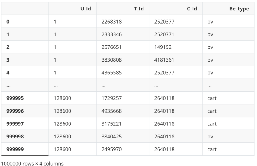
df = data.head(1000000)
df.head(1)
.dataframe tbody tr th {
    vertical-align: top;
}
.dataframe thead th {
    text-align: right;
}
Analysis of user traffic and purchase time
User behavior statistics
describe = df.loc[:,["U_Id","Be_type"]]
ids = pd.DataFrame(np.zeros(len(set(list(df["U_Id"])))),index=set(list(df["U_Id"])))
pv_class=describe[describe["Be_type"]=="pv"].groupby("U_Id").count()
pv_class.columns = ["pv"]
buy_class=describe[describe["Be_type"]=="buy"].groupby("U_Id").count()
buy_class.columns = ["buy"]
fav_class=describe[describe["Be_type"]=="fav"].groupby("U_Id").count()
fav_class.columns = ["fav"]
cart_class=describe[describe["Be_type"]=="cart"].groupby("U_Id").count()
cart_class.columns = ["cart"]
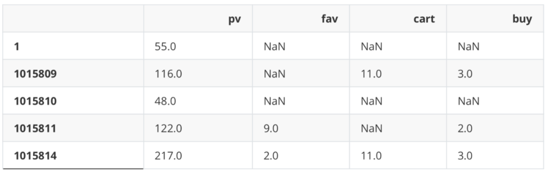
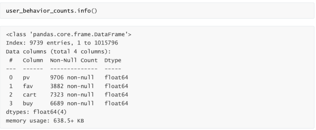
user_behavior_counts=ids.join(pv_class).join(fav_class).join(cart_class).join(buy_class).
iloc[:,1:]
user_behavior_counts.head()
.dataframe tbody tr th {
    vertical-align: top;
}
.dataframe thead th {
    text-align: right;
}
Time change analysis of total traffic volume (days)
from matplotlib import font_manager
# Solve the confusion of negative sign of coordinate axis scale
# Resolve minus sign'-'Questions displayed as squares plt.rcParams['axes.unicode_minus'] = False # Solve the Chinese garbled code problem PLT rcParams['font.sans-serif'] = ['Simhei']
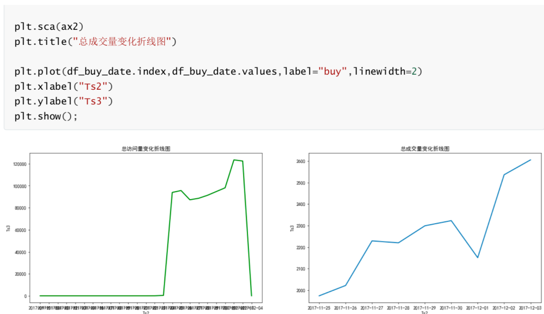
According to the analysis of the time change of total traffic and trading volume, there was a slight fluctuation in traffic and trading volume from November 25, 2017 to December 1, 2017. The traffic and trading volume increased significantly on December 2, 2017, and maintained high traffic and trading volume on December 2 and 3. One of the reasons for this phenomenon is that December 2 and 3 are weekends. At the same time, considering that there may be some promotional activities on December 2 and 3, it can be analyzed in combination with the actual business situation. (in the figure, the number of visitors increased on Friday, but the trading volume decreased. It is speculated that this phenomenon may be related to the postponement of trading on Friday caused by weekend activities.)
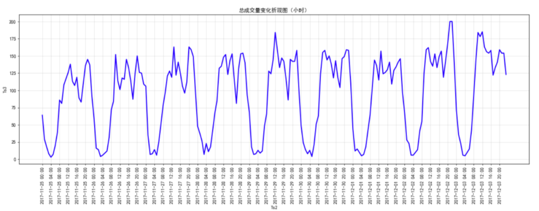
Time change analysis of total traffic volume (hours)
# Data preparation df_pv_timestamp=df[df["Be_type"]=="pv"][["Be_type","Ts1"]] df_pv_timestamp["Ts1"] = pd.to_datetime(df_pv_timestamp["Ts1"])
df_pv_timestamp=df_pv_timestamp.set_index("Ts1")
df_pv_timestamp=df_pv_timestamp.resample("H").count()["Be_type"]
df_pv_timestamp
df_buy_timestamp=df[df["Be_type"]=="buy"][["Be_type","Ts1"]]
df_buy_timestamp["Ts1"] = pd.to_datetime(df_buy_timestamp["Ts1"])
df_buy_timestamp=df_buy_timestamp.set_index("Ts1")
df_buy_timestamp=df_buy_timestamp.resample("H").count()["Be_type"]
df_buy_timestamp
Ts1
2017-09-11 16:00:00        1
2017-09-11 17:00:00        0
2017-09-11 18:00:00        0
2017-09-11 19:00:00        0
2017-09-11 20:00:00        0
                       ...
2017-12-03 20:00:00     8587
2017-12-03 21:00:00    10413
2017-12-03 22:00:00     9862
2017-12-03 23:00:00     7226
2017-12-04 00:00:00        1
Freq: H, Name: Be_type, Length: 2001, dtype: int64
Ts1
2017-11-25 00:00:00     64
2017-11-25 01:00:00     29
2017-11-25 02:00:00     18
2017-11-25 03:00:00      8
2017-11-25 04:00:00      3
                      ...
2017-12-03 19:00:00    141
2017-12-03 20:00:00    159
2017-12-03 21:00:00    154
2017-12-03 22:00:00    154
2017-12-03 23:00:00    123
Freq: H, Name: Be_type, Length: 216, dtype: int64
#mapping
plt.figure(figsize=(20,6),dpi =70)
x2= df_buy_timestamp.index plt.plot(range(len(x2)),df_buy_timestamp.values,label="Turnover",color="blue",linewidth=2) plt.title("Discount chart of total trading volume change(hour)")
x2 = [i.strftime("%Y-%m-%d %H:%M") for i in x2]
plt.xticks(range(len(x2))[::4],x2[::4],rotation=90)
plt.xlabel("Ts2")
plt.ylabel("Ts3")
plt.grid(alpha=0.4);
Characteristic Engineering
Idea: regardless of the time window, only the user's click, collection and other behaviors are used to predict the purchase process: take the user ID(U_Id) as the grouping key, and count the click, collection and shopping cart behaviors of each user, respectively:
Whether to click and the number of clicks; Collection or not, collection times; Whether to add shopping cart and the number of times to add shopping cart
So as to predict whether to buy in the end
# Remove timestamp
df = df[["U_Id", "T_Id", "C_Id", "Be_type"]] df
.dataframe tbody tr th {
    vertical-align: top;
}
.dataframe thead th {
    text-align: right;
}
Behavior type
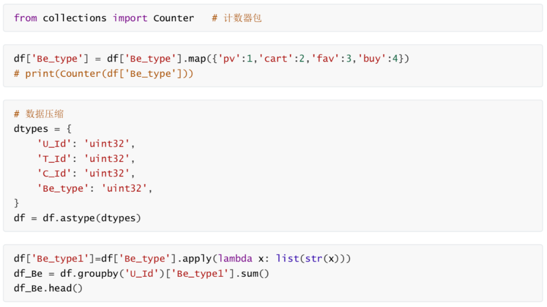
U_Id
1 [1,1,1,1,1,1,1,1,1,1,1,1,1,1,1,...
100 [1,1,1,1,1,1,1,1,1,3,1,1,3,1,3,...
115 [1,1,1,1,1,1,1,1,1,1,1,1,1,1,3,...
117 [4,1,1,1,1,1,1,4,1,1,1,1,1,1,1,...
118 [1,1,1,1,1,1,1,1,1,1,1,1,1,1,1,...
Name: Be_type1, dtype: object
Finally, create a DataFrame to store the calculated user behavior.
df_new = pd.DataFrame()
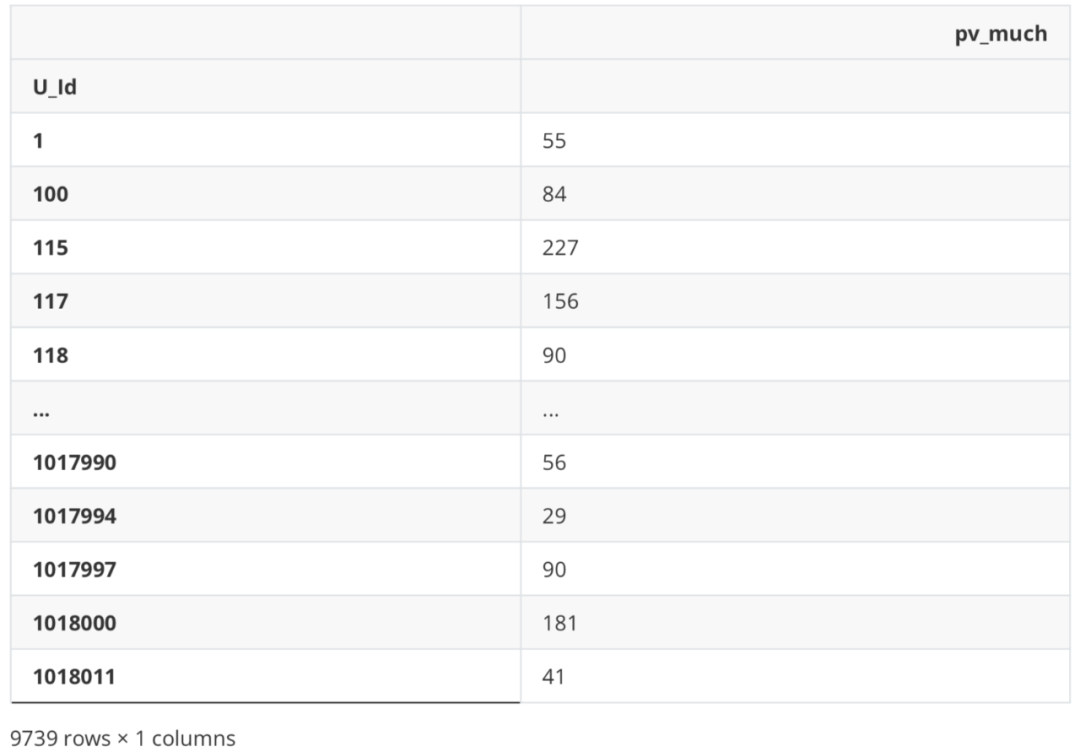
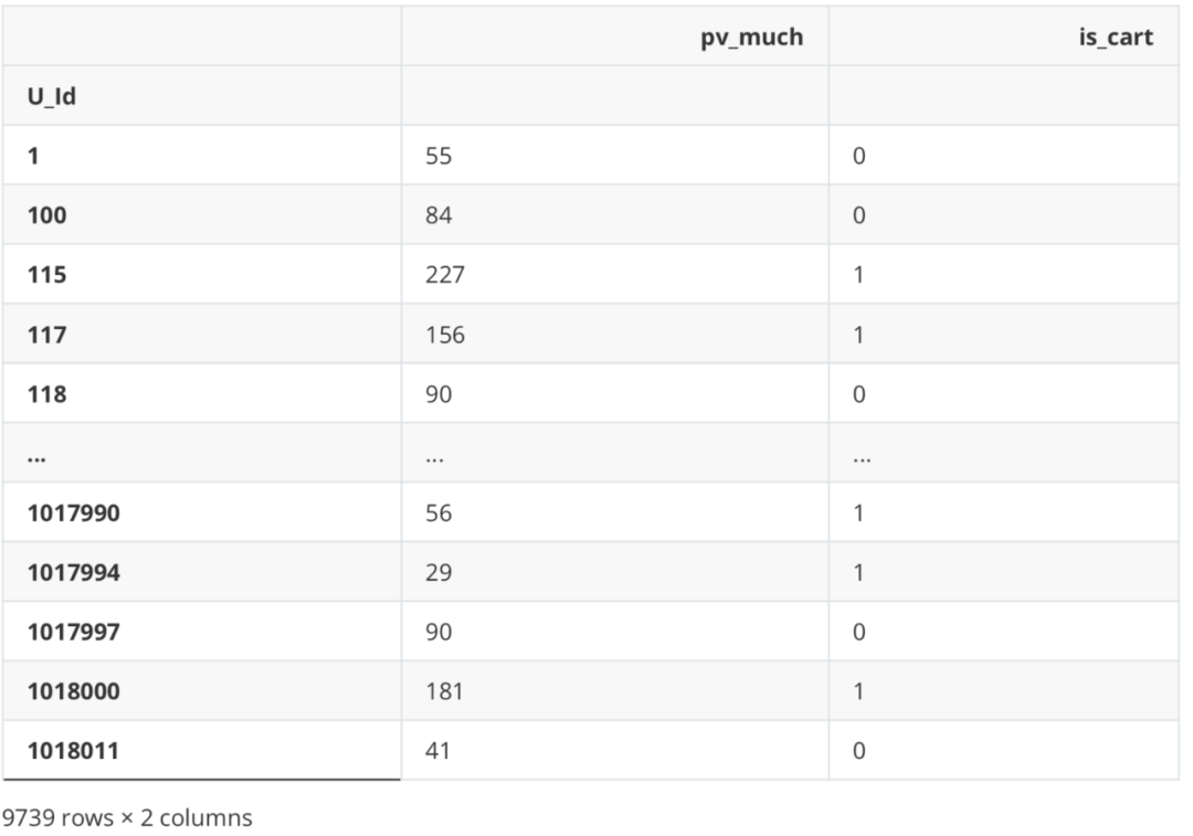
Number of hits
df_new['pv_much'] = df_Be.apply(lambda x: Counter(x)['1'])
df_new
.dataframe tbody tr th {
    vertical-align: top;
}
.dataframe thead th {
    text-align: right;
}
Additional purchase times
#Add purchase or not
df_new['is_cart'] = df_Be.apply(lambda x: 1 if '2' in x else 0)
df_new
.dataframe tbody tr th {
    vertical-align: top;
}
.dataframe thead th {
    text-align: right;
}
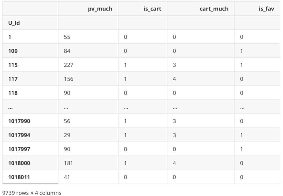
#Several additional purchases
df_new['cart_much'] = df_Be.apply(lambda x: 0 if '2' not in x else Counter(x)['2'])
df_new
.dataframe tbody tr th {
    vertical-align: top;
}
.dataframe thead th {
    text-align: right;
}

Collection times
#Collect
df_new['is_fav'] = df_Be.apply(lambda x: 1 if '3' in x else 0)
df_new
.dataframe tbody tr th {
    vertical-align: top;
}
.dataframe thead th {
    text-align: right;
}
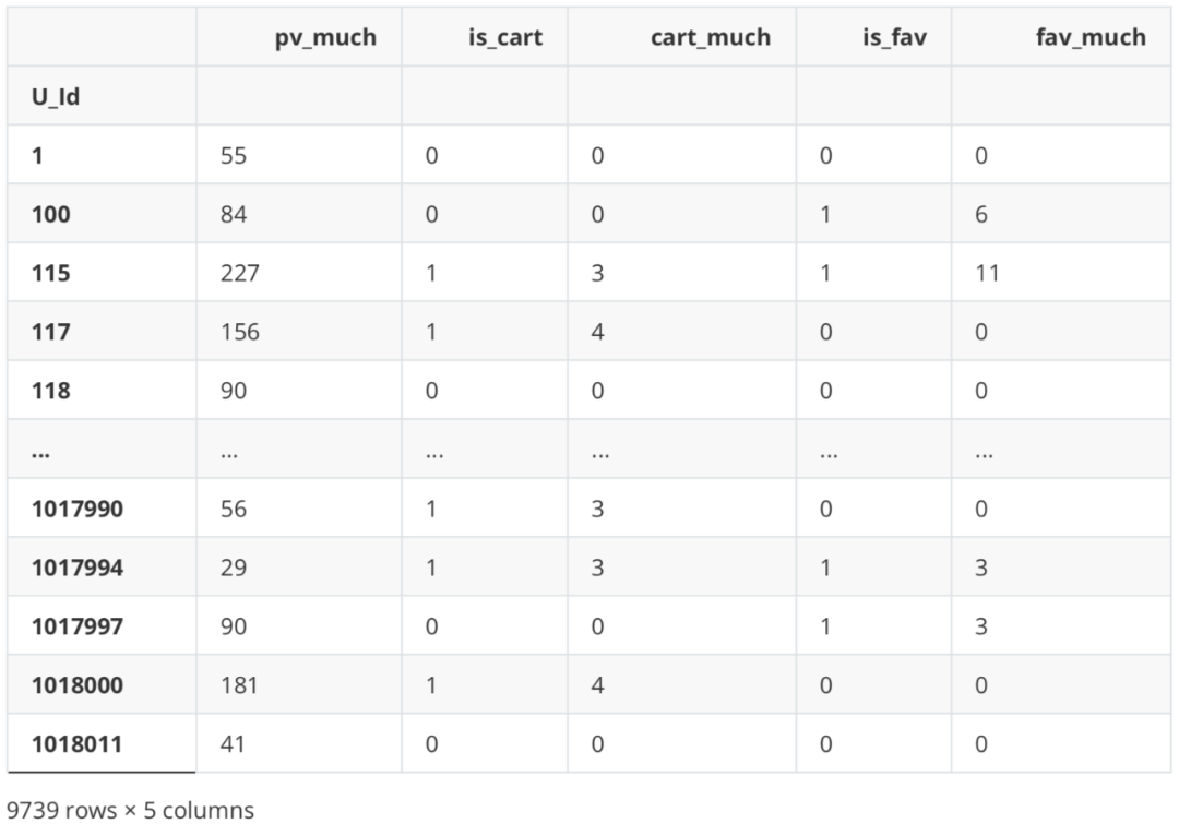
#Collected several times
df_new['fav_much'] = df_Be.apply(lambda x: 0 if '3' not in x else Counter(x)['3'])
df_new
.dataframe tbody tr th {
    vertical-align: top;
}
.dataframe thead th {
    text-align: right;
}
correlation analysis
#Partial data df_new.corr('spearman')
.dataframe tbody tr th {
    vertical-align: top;
}
.dataframe thead th {
    text-align: right;
}
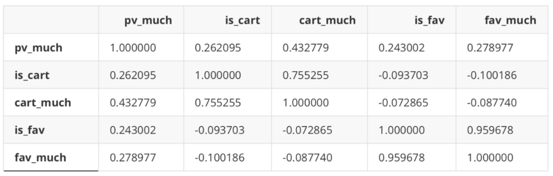
There is a certain correlation between the number of additional purchases and the number of additional purchases, and between the number of collections and the number of collections. However, it is verified that the effect of eliminating one of them is basically the same as that of including all variables, so all variables are used for modeling later.
Data label
import seaborn as sns
#Buy or not
df_new['is_buy'] = df_Be.apply(lambda x: 1 if '4' in x else 0)
df_new
.dataframe tbody tr th {
    vertical-align: top;
}
.dataframe thead th {
    text-align: right;
}
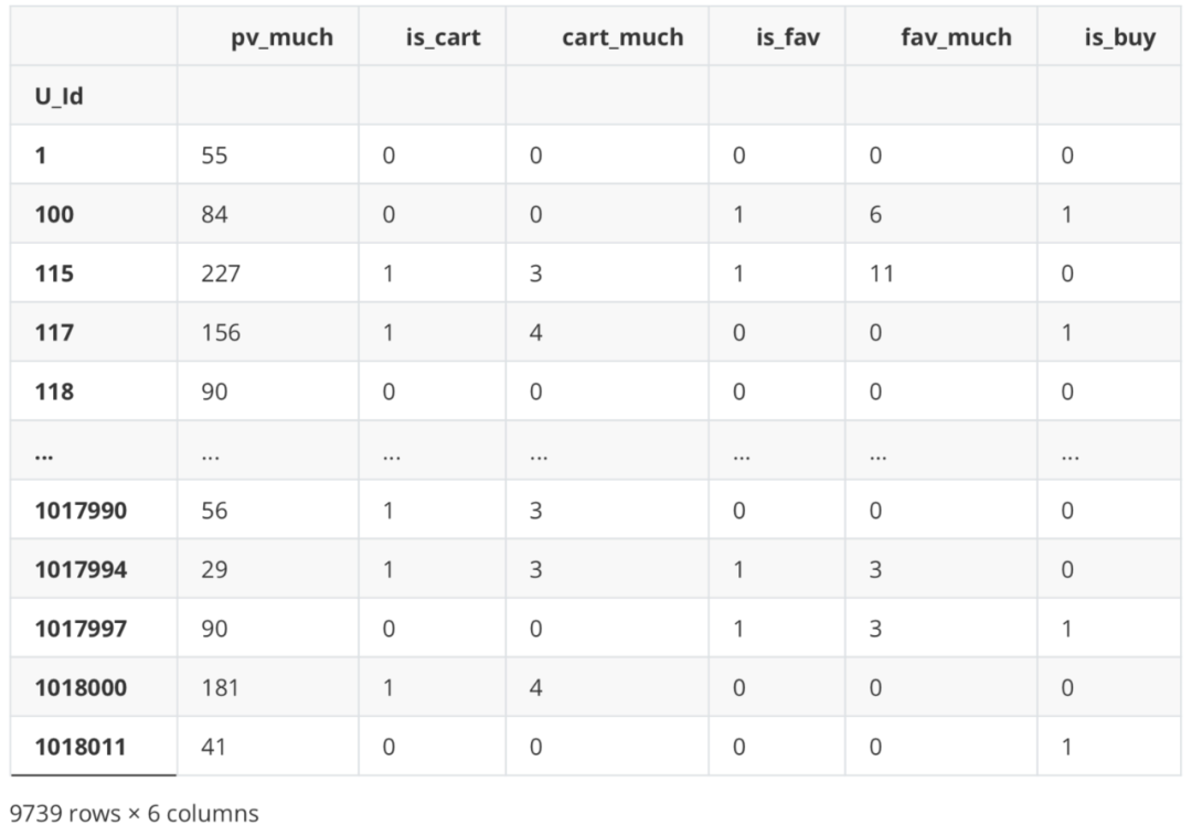
df_new.is_buy.value_counts()
1    6689
0    3050
Name: is_buy, dtype: int64
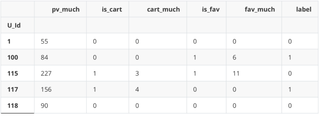
df_new['label'] = df_new['is_buy']
del df_new['is_buy']
df_new.head()
.dataframe tbody tr th {
    vertical-align: top;
}
.dataframe thead th {
    text-align: right;
}
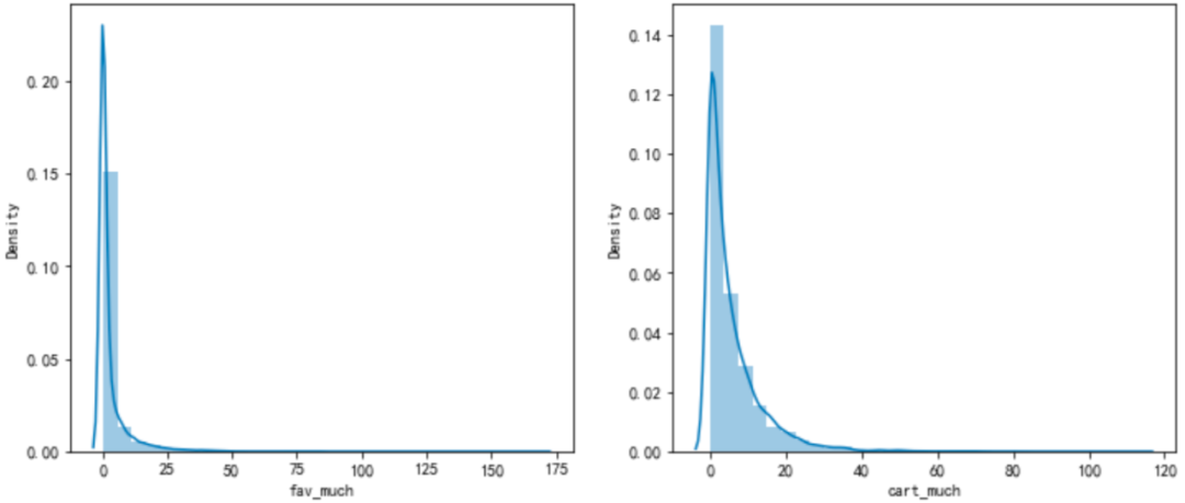
f,ax=plt.subplots(1,2,figsize=(12,5))
sns.set_palette(["#9b59b6","#3498db",]) #Set the colors of all graphs and use hls color space
sns.distplot(df_new['fav_much'],bins=30,kde=True,label='123',ax=ax[0]);
sns.distplot(df_new['cart_much'],bins=30,kde=True,label='12',ax=ax[1]);
C:\Users\CDA\anaconda3\lib\site-packages\seaborn\distributions.py:2619: FutureWarning:
`distplot` is a deprecated function and will be removed in a future version. Please adapt
your code to use either `displot` (a figure-level function with similar flexibility) or
`histplot` (an axes-level function for histograms).
  warnings.warn(msg, FutureWarning)
C:\Users\CDA\anaconda3\lib\site-packages\seaborn\distributions.py:2619: FutureWarning:
`distplot` is a deprecated function and will be removed in a future version. Please adapt
your code to use either `displot` (a figure-level function with similar flexibility) or
`histplot` (an axes-level function for histograms).
warnings.warn(msg, FutureWarning)
Model building
Partition dataset
from sklearn.model_selection import train_test_split
X = df_new.iloc[:,:-1]
Y = df_new.iloc[:,-1]
X.head()
Y.head()
.dataframe tbody tr th {
    vertical-align: top;
}
.dataframe thead th {
    text-align: right;
}
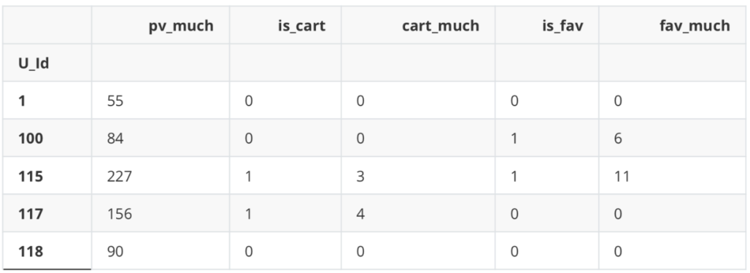
U_Id
10
100 1
115 0
117 1
118 0
Name: label, dtype: int64
Xtrain,Xtest,Ytrain,Ytest = train_test_split(X,Y,test_size= 0.3,random_state= 42)
logistic regression
Model establishment
from sklearn.linear_model import LogisticRegression
LR_1 = LogisticRegression().fit(Xtrain,Ytrain)
#Simple test LR_1.score(Xtest,Ytest)
0.6741957563312799
Model evaluation
from sklearn import metrics
from sklearn.metrics import classification_report
from sklearn.metrics import auc,roc_curve
#Confusion matrix
print(metrics.confusion_matrix(Ytest, LR_1.predict(Xtest)))
[[   0  952]
 [   0 1970]]
print(classification_report(Ytest,LR_1.predict(Xtest)))
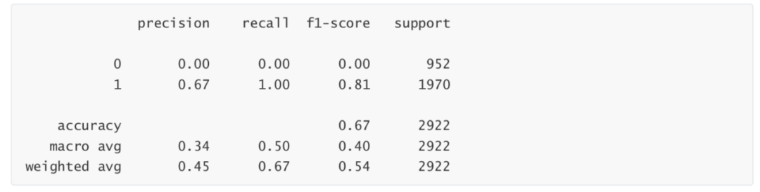
D:\anaconda\lib\site-packages\sklearn\metrics\_classification.py:1308:
UndefinedMetricWarning: Precision and F-score are ill-defined and being set to 0.0 in
labels with no predicted samples. Use `zero_division` parameter to control this behavior.
  _warn_prf(average, modifier, msg_start, len(result))
fpr,tpr,threshold = roc_curve(Ytest,LR_1.predict_proba(Xtest)[:,1])
roc_auc = auc(fpr,tpr)
print(roc_auc)
0.6379193682549162
Random forest
Model establishment
from sklearn.ensemble import RandomForestClassifier
rfc = RandomForestClassifier(n_estimators=200, max_depth=1)
rfc.fit(Xtrain, Ytrain)
RandomForestClassifier(max_depth=1, n_estimators=200)
Model evaluation
#Confusion matrix
print(metrics.confusion_matrix(Ytest, rfc.predict(Xtest)))
[[   0  952]
 [   0 1970]]
#Classification Report
print(metrics.classification_report(Ytest, rfc.predict(Xtest)))
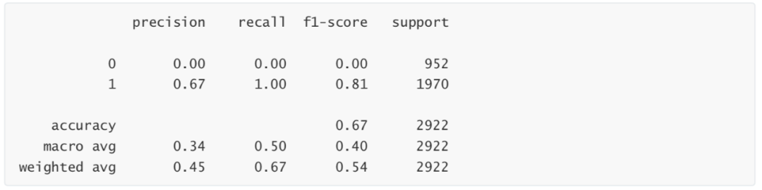
D:\anaconda\lib\site-packages\sklearn\metrics\_classification.py:1308:
UndefinedMetricWarning: Precision and F-score are ill-defined and being set to 0.0 in
labels with no predicted samples. Use `zero_division` parameter to control this behavior.
  _warn_prf(average, modifier, msg_start, len(result))