Original author: King James, master of data science, King's College London
Original address:[ Portal]

preface

For entry into machine learning, you must understand the gradient descent method. Although the gradient descent method is not directly used in machine learning, understanding the thinking of gradient descent method is the basis for subsequent learning of other algorithms. There are many articles on the Internet about gradient descent method. But most articles are either a whole pile of mathematical formulas, or simply drop in the opposite direction of the gradient. This article is easy to understand and explain. You can understand it with high school mathematics knowledge.

1. Introduction

Let's start with a case. The figure below shows a group of house price information in Jing'an District, Shanghai

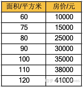
(don't look, I made up the data. The house price in Jing'an District of Shanghai can't be so cheap)

We use Python to draw the following figure on the coordinate system:

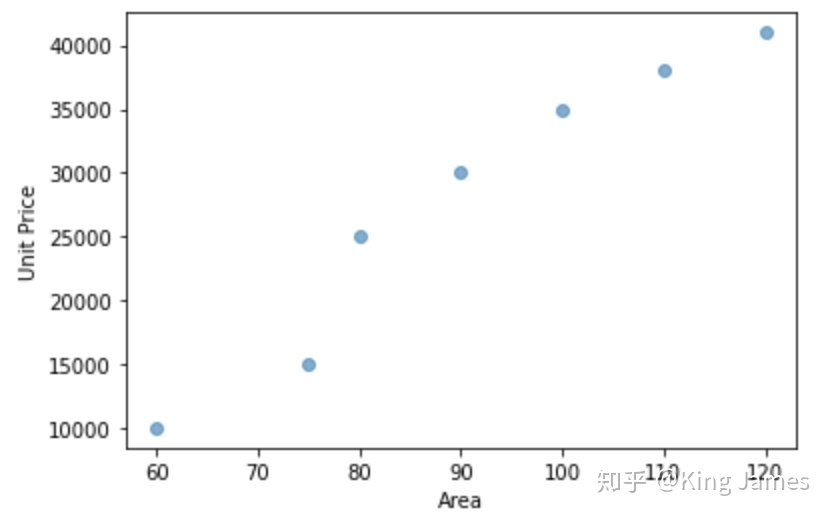
We now want to fit a linear function to express the relationship between house area and house price. The expression of univariate primary function we learned in junior middle school is: y=kx+b (K ≠ 0). Obviously, it is impossible for a pair of combinations (k,b) to pass through the seven points in the figure above. We can only find a pair of combinations as far as possible, so that the linear function is closest to the total distance of the seven points in the figure above.

As shown in the figure above, the mean square deviation of the difference between the actual value and the predicted value is called loss function, or cost function or cost function, which has the same meaning. We hope to find a combination (k, b) that can minimize the value of the loss function. There is only one input variable x above. If we add more input variables, such as the number of bedrooms and the distance from the nearest subway station. The final objective variable and loss function are expressed by the following function expression:

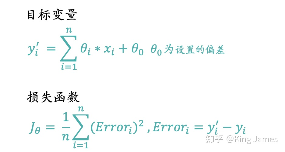
Now our task is to find a group θ， The value of the loss function is minimized on the premise that [x, y] is known. So how to calculate θ Yes, what method is used?

Let's first go back to the loss function expression itself. The loss function itself is a form of y=x^2. Everyone should have learned mathematics in senior high school. This is a parabolic equation with an opening upward, which is roughly as follows:

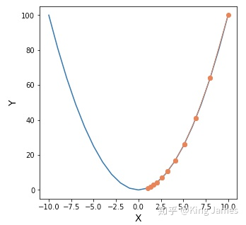
How do we find the lowest point of this function? The above figure is a two-dimensional diagram. We can easily see with the naked eye that when x=0, y is the smallest. If there are more dimensions, such as z = (x-10)^2 + (y-10)^2, the following figure is obtained:

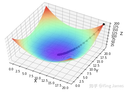
How do we locate the minimum value? In particular, x here is a concept of "large" parameter, and x should be equal to the following formula

Let's make it clear that the abscissa in the figure above is x and Y in the function expression θ We already know, so we find the most appropriate (x,y) to minimize the value of the function. If we are now a known sample (x,y), then the variable in the figure above becomes θ 0 θ_0 θ 0} and θ i θ_i θ i, not really x i x_i xi, we are θ 0 θ_0 θ 0} and θ i θ_i θ i) diagram as input variable, x i x_i xi. And y i y_i yi ， are known fixed values, which must be clear. The value of the ordinate in the figure above becomes the value of the loss function.

Our problem is to know the coordinates (x,y) of the sample to solve a set of problems θ Parameter to minimize the value of the loss function. How do we find the lowest point in the figure above? Because we find the lowest point, all dimensions of the abscissa corresponding to the lowest point are what we want θ 0 θ_0 θ 0} and θ i θ_i θ i, and the ordinate is the minimum value of the loss function. Find the lowest point and all the answers will be solved.

Now the problem? Is there an algorithm that allows us to slowly locate the minimum value? This algorithm is the gradient descent method.

2. Introduction to gradient descent method

2.1 idea of gradient descent method

Firstly, we introduce the overall idea of gradient descent method. Suppose you are standing at the top of a mountain. You have to reach the lowest point of the mountain before dark. There is a food and water supply station where you can supplement energy. You don't need to consider the safety of going down the mountain. Even if you choose the steepest cliff, you can retreat all over. So how can you go down the mountain fastest?

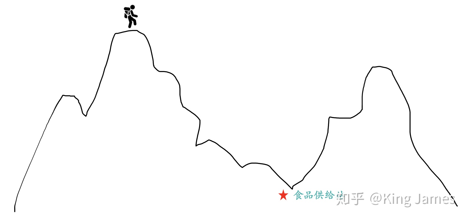
The quickest way is to take the current position as the benchmark, find the steepest place in the position, and then go down in that direction. After walking a certain distance, we can find the steepest place again based on the current position, repeat it all the time, and finally we can reach the lowest point. We need to constantly reposition the steepest place so that it is not limited to local optimization.

Then we will face two problems in the whole process of going down the mountain:

How to measure the "steepness" of mountain peaks;
Measure the steepness again after each distance; If you go too long, the overall measurement times will be less, which may lead to not taking the best route and missing the lowest point. The journey is too short, the measurement times are too frequent, and the overall time is too long. It has already GG before reaching the food supply station. How to set the step size here?

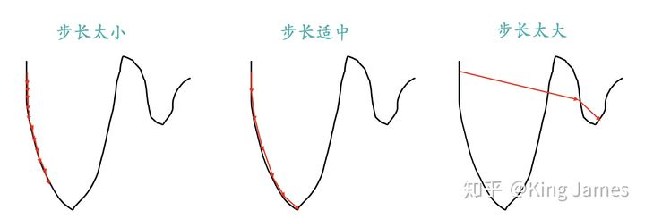
Part 1 describes how to locate the highest point of a parabola from an opening upward to the lowest point, which is completely similar to the scene of going down the mountain. The parabola is equivalent to a mountain peak. Our goal is to find the lowest point of the parabola, that is, the bottom of the mountain. The fastest way to go down the mountain is to find the steepest direction of the current position, and then go down this direction. Corresponding to the parabola, it is to calculate the gradient of a given point, and then move in the opposite direction of the gradient (Part 2.3 will explain why it is in the opposite direction of the gradient), so as to make the parabola value drop the fastest. At the same time, like going down the mountain, we should constantly locate the new position, calculate the gradient of the new position, then descend in the new direction, and finally slowly locate the lowest point of the parabola.

2.2 gradient descent algorithm

Part2. The idea of gradient descent method has been introduced, leaving two problems. The first is how to calculate the "steepness". We call it gradient here. We use ≓ J_ θ Instead. The second is the step size problem. We use one α The learning rate represents this step, α Larger represents larger step size. Knowing these two values, how do we get them θ Parameter update expression?

J is about θ A function that assumes that initially we are θ_ 1 at this position, go from this point to the minimum point of J, that is, the bottom of the mountain. First, we determine the forward direction, that is, the reverse of the gradient "- J_ θ”， Then walk a distance in steps, that is α， After this step, we will arrive at θ_ 2 this point. The expression is as follows:

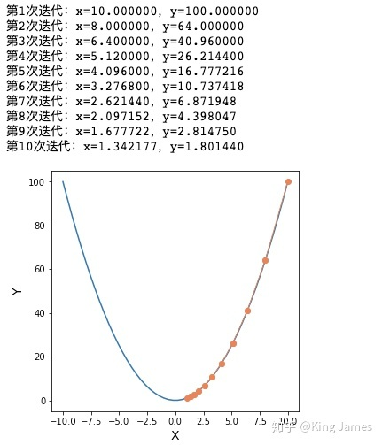
We keep updating according to the above expression θ Value until θ Until the convergence remains unchanged, when we reach the bottom of the mountain, the gradient of the function is 0, θ The value will not be updated because the second half of the expression is always 0. The value of the loss function must be decreasing during the whole descent process, but we want to learn the parameter value θ Not necessarily decreasing all the time. Because we need to find the coordinate point with the smallest loss function. The coordinates of this coordinate point are not necessarily the origin, but may be (2, 3) or even (4, 6). What we find is the most appropriate θ Value minimizes the loss function. In the following figure, we use an example to illustrate:


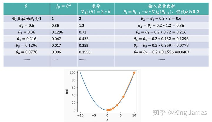
The lowest point in the figure above is obviously the origin. We approach this lowest point by gradient descent method. We can see that the value of the loss function is decreasing all the time, θ The value of is also converging towards the value of 0.

2.3 mathematical calculation of gradient descent method

Part2.1 and 2.2 introduce the idea and method of gradient descent θ The updated expression is now explained mathematically:

• Why does it fall in the opposite direction of the gradient:
  
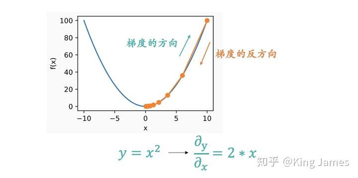
  The figure above should vividly show why it is moving in the opposite direction of the gradient. The gradient is a vector, and the direction of the gradient is the fastest rising direction of the function at the specified point, so the opposite direction of the gradient is naturally the fastest falling direction.

• Generic θ Parameter update formula:
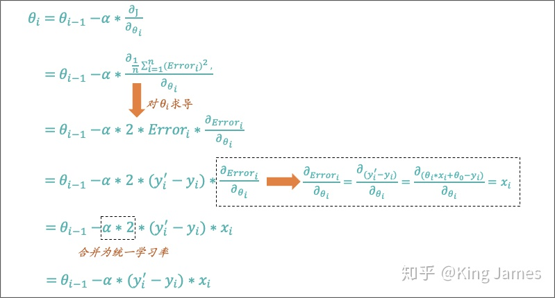
  Part2. In the example in 2, we choose the simplest function expression, θ There are two kinds of parameters. One is the parameter paired with the input variable x θ_ i. One is a fixed deviation θ_ 0 We use the known sample data (x,y) to solve a set of problems that minimize the loss function θ Parameters. Let's calculate a general generalization θ Parameter update expression. We only need to use the derivative knowledge in high school mathematics. My friends believe I'm really easy.
  The following figure shows the parameters paired with the input variable x θ_ i update expression:
  
  The following figure shows the deviation from the fixed θ_ Update expression for 0:
  
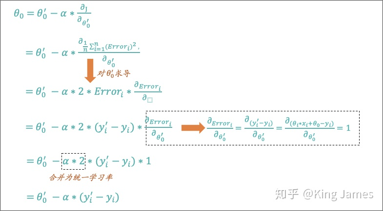
  The above mathematical process is the simplest derivative process in high school. So far, we have introduced the idea and mathematical explanation of gradient descent algorithm.

2.4 gradient descent classification

Part2. You can also see the formula in 3. We need to use the (x, y) data of the sample to calculate the parameters θ If there are 100 pieces of data in the sample, how can we update it. Under normal circumstances, we update in two ways:

• Stochastic gradient descent
  We use only a single training sample to update each time θ Parameters, traversing the training set in turn, rather than considering all samples in one update. Just like the seven house price data introduced at the beginning, we calculate them one by one and update them once θ， until θ The convergence or post update range has been less than the threshold we set.

• Batch gradient descent
  Each update traverses all samples in the training set and updates based on the sum of their prediction errors. We will summarize the prediction errors of 7 sample data at one time, and then update them once. After updating, continue to summarize with the sum of prediction errors of 7 sample data, and then update until θ The convergence or post update range has been less than the threshold we set.

When the number of training samples is large, each update of batch gradient descent will be an operation with a large amount of calculation, and random gradient descent can be updated immediately by using a single training sample, so random gradient descent is usually a faster method. But random gradient descent also has a disadvantage, that is θ It may not converge, but oscillate near the minimum, but it will get a good enough approximation in practice. Therefore, in practice, we generally do not need a fixed learning rate, but let it gradually reduce to zero with the operation of the algorithm, that is, when approaching the "bottom of the mountain", slowly reduce the falling "stride" and replace it with "small broken steps", so that it is easier to converge to the global minimum rather than oscillate around it.

3. Practice of gradient descent method

3.1 univariate: y = x^2 find the lowest point

import matplotlib.pyplot as plt
import numpy as np
# Function value of fx
def fx(x):
    return x**2

#Define gradient descent algorithm
def gradient_descent():
    times = 10 # Number of iterations
    alpha = 0.1 # Learning rate
    x =10# Set the initial value of x
    x_axis = np.linspace(-10, 10) #Sets the coordinate system of the x axis
    fig = plt.figure(1,figsize=(5,5)) #Set canvas size
    ax = fig.add_subplot(1,1,1) #Set that there is only one graph in the canvas
    ax.set_xlabel('X', fontsize=14)
    ax.set_ylabel('Y', fontsize=14)
    ax.plot(x_axis,fx(x_axis)) #Mapping
    
    for i in range(times):
        x1 = x          
        y1= fx(x)  
        print("Number%d Iterations: x=%f，y=%f" % (i + 1, x, y1))
        x = x - alpha * 2 * x
        y = fx(x)
        ax.plot([x1,x], [y1,y], 'ko', lw=1, ls='-', color='coral')
    plt.show()

if __name__ == "__main__":
    gradient_descent()

3.2 multivariable: z = (x-10)^2 + (y-10)^2 find the lowest point

import matplotlib.pyplot as plt
import numpy as np
from mpl_toolkits.mplot3d import Axes3D
#Find the function value of fx
def fx(x, y):
    return (x - 10) ** 2 + (y - 10) ** 2

def gradient_descent():
    times = 100 # Number of iterations
    alpha = 0.05 # Learning rate
    x = 20 # Initial value of x
    y = 20 # Initial value of y

    fig = Axes3D(plt.figure()) # Set canvas to 3D
    axis_x = np.linspace(0, 20, 100)#Set the value range of X axis
    axis_y = np.linspace(0, 20, 100)#Set the value range of Y axis
    axis_x, axis_y = np.meshgrid(axis_x, axis_y) #Convert data to grid data
    z = fx(axis_x,axis_y)#Calculate Z-axis value
    fig.set_xlabel('X', fontsize=14)
    fig.set_ylabel('Y', fontsize=14)
    fig.set_zlabel('Z', fontsize=14)
    fig.view_init(elev=60,azim=300)#Set the top view angle of 3D graph to facilitate viewing the gradient descent curve
    fig.plot_surface(axis_x, axis_y, z, rstride=1, cstride=1, cmap=plt.get_cmap('rainbow')) #Make base map
    
    for i in range(times):
        x1 = x        
        y1 = y         
        f1 = fx(x, y)  
        print("Number%d Iterations: x=%f，y=%f，fxy=%f" % (i + 1, x, y, f1))
        x = x - alpha * 2 * (x - 10)
        y = y - alpha * 2 * (y - 10)
        f = fx(x, y)
        fig.plot([x1, x], [y1, y], [f1, f], 'ko', lw=2, ls='-')
    plt.show()

if __name__ == "__main__":
    gradient_descent()

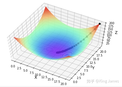
3.3 find the best solution according to the given sample θ combination

import numpy as np
import matplotlib.pyplot as plt   
#sample data 
x = [1,2,3,4,5,6,7,8,9,10,11,12,13,14,15,16,17,18,19,20]
y = [3,4,5,5,2,4,7,8,11,8,10,11,13,13,16,17,16,17,18,20]
m = 20 #Number of samples
alpha = 0.01#Learning rate
θ_0 = 1 #initialization θ_ Value of 0
θ_1 = 1 #initialization θ_ Value of 1

#Predict the value of the target variable y
def predict(θ_0,θ_1, x):
    y_predicted = θ_0 + θ_1*x
    return y_predicted

#Traverse the entire sample data, calculate the deviation, and use the batch gradient descent method
def loop(m,θ_0,θ_1,x,y):
    sum1 = 0
    sum2 = 0
    error = 0
    for i in range(m):
        a = predict(θ_0,θ_1, x[i]) - y[i]
        b = (predict(θ_0,θ_1, x[i]) - y[i])* x[i]
        error1 = a*a
        sum1 = sum1 + a
        sum2 = sum2 + b
        error = error + error1
    return sum1,sum2,error

#Batch gradient descent method for updating θ Value of
def batch_gradient_descent(x, y,θ_0,θ_1, alpha,m):
    gradient_1 = (loop(m,θ_0,θ_1,x,y)[1]/m)
    while abs(gradient_1) > 0.001:#Set a threshold value. When the absolute value of the gradient is less than 0.001, it will not be updated
        gradient_0 = (loop(m,θ_0,θ_1,x,y)[0]/m)
        gradient_1 = (loop(m,θ_0,θ_1,x,y)[1]/m)
        error = (loop(m,θ_0,θ_1,x,y)[2]/m)
        θ_0 = θ_0 - alpha*gradient_0
        θ_1 = θ_1 - alpha*gradient_1
    return(θ_0,θ_1,error)

θ_0 = batch_gradient_descent(x, y,θ_0,θ_1, alpha,m)[0]
θ_1 = batch_gradient_descent(x, y,θ_0,θ_1, alpha,m)[1]
error = batch_gradient_descent(x, y,θ_0,θ_1, alpha,m)[2]
print ("The θ_0 is %f, The θ_1 is %f, The The Mean Squared Error is %f " %(θ_0,θ_1,error))

plt.figure(figsize=(6, 4))# Create a new canvas
plt.scatter(x, y, label='y')# Draw sample scatter diagram
plt.xlim(0, 21)# x-axis range
plt.ylim(0, 22)# y-axis range
plt.xlabel('x', fontsize=20)# x-axis label
plt.ylabel('y', fontsize=20)# y-axis label

x = np.array(x)
y_predict = np.array(θ_0 + θ_1*x)
plt.plot(x,y_predict,color = 'red')#Draw the function diagram of fitting
plt.show()

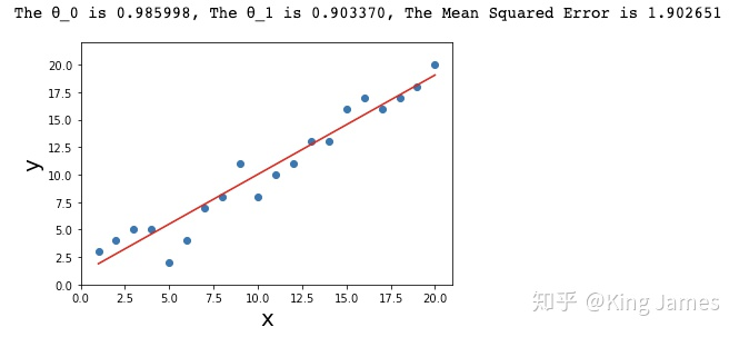
In the first half of this article, the whole gradient descent algorithm is explained in a comprehensive way. In the second half, the whole algorithm is implemented in Python. You can download and run it yourself. Welcome to communicate ~